The optical time-domain reflectometer (OTDR) is used to characterize a fiber optic span. It performs single-ended tests and can calculate fiber attenuation and uniformity and splice and connector losses. It can also locate breaks and determine fiber length. Its ability to locate and measure reflectance and loss makes it the troubleshooting and fault locating equipment of choice. New generation OTDRs include advanced functions such as macrobend location, active-fiber testing and automatic trace acquisition.
Michel Leclerc and Vincent Racine, EXFO
An optical time-domain reflectometer sends short pulses of light into a fiber and measures its reflections as a function of time. The delay of these reflections to the detector as well as their intensity tells the story of the fiber link itself. This time lapse between pulse launch and detection, in relation to the speed of light in the glass material, allows distances to be calculated and events to be characterized. An OTDR calculates distance as:
d = (c × t)/2(IOR)
where c is the speed of light, t the round-trip travel time and IOR the index of refraction of the fiber under test as specified by the manufacturer.
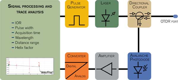
Figure 1. Lasers and detectors are key elements in an OTDR.
An OTDR comprises a microprocessor, a pulse trigger and generator, a laser diode, an optical coupler, a detector, an analog-to-digital converter and a display (Figure 1). When the test button is pressed, the microprocessor sends a set of instructions to the trigger and generator that tells the laser to send a pulse. The pulses then pass through the directional optical coupler to the OTDR port and into the fiber being tested.
Typically, an OTDR will be equipped with two, three or even four lasers, specified at the main transmission windows. When testing multimode fiber, these windows are located around 850 and 1300 nm. For single-mode fiber, they are around 1310 and 1550 nm. OTDRs designed for specific applications, such as fiber-to-the-home (FTTH), also include the 1490 nm wavelength.
Legacy OTDRs are designed to test inactive fibers — also called dark fibers — and are normally used during the construction phase or when troubleshooting fiber sections that are not carrying traffic. New generation OTDRs can offer filtered ports, designed to measure fibers that are carrying live traffic signals, i.e., active fibers. A live-fiber-testing OTDR uses a laser generating at 1625 or 1650 nm and a filter, which prevents transmission wavelengths from interfering with the OTDR’s optical components.
As the pulse travels down the fiber, two phenomena occur: Rayleigh scattering and Fresnel reflections. Rayleigh scattering results from minute variations in fiber density such as inconsistencies in the index of refraction. Small amounts of light reflect from each point in the fiber toward the transmitter. Fresnel reflections occur when the light traveling down the fiber encounters abrupt changes in material density that may occur at connections or breaks where an air gap exists. A large amount of light, compared with the Rayleigh scattering, is reflected. The strength of the reflection depends upon the degree of change in density.
The returning signal, therefore, consists of both Rayleigh scattering and Fresnel reflections. The power level of the Fresnel reflection is tens of thousands of times stronger than the Rayleigh scattering. At the OTDR, the optical coupler directs the reflected signal away from the originating laser and into the detector (either avalanche photodiode or PIN). The signal passes through the analog-to-digital converter to the microprocessor for analysis and display.
The processor then averages the data to improve the signal-to-noise ratio and displays the points that make up the fiber trace or waveform (Figure 2). The trace is a collection of tens of thousands of sampling points. Because of the OTDR’s limited display resolution, not all of these data points can be displayed on screen at the same time. When the full trace is being displayed, each point on the screen represents an average of a dozen sampling points.
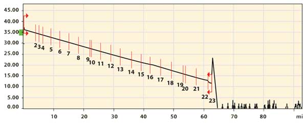
Figure 2. A typical OTDR trace comprises tens of thousands of sampling points.
An OTDR’s performance can be accurately evaluated by briefly examining the following key specifications:
Dynamic range describes the loss and distance measurement capability. Measured in decibels, it is the difference between the backscatter level at the front end of the fiber and the noise floor at the end of the fiber. Because the length of the pulse width determines how much optical energy is injected into the fiber, larger pulse widths correspond to greater dynamic range specifications.
Measurement range is defined by Bellcore as the maximum attenuation that can be placed between the OTDR and the event being measured, and still allow measurement within acceptable accuracy limits. Therefore, the OTDR must be able to see and measure the loss of an event within the specified measurement range.
Dead zones result from a temporary blinding of the detector following a reflective event. They occur when the high return power from Fresnel reflections saturates the detector, and they are associated with every reflective event. An OTDR cannot detect or measure events in the dead zone.
Event (or reflective) and attenuation (or nonreflective) are the two main types of dead zones. The event dead zone represents the minimum distance between the beginning of a reflective event and the point where a consecutive reflective event can be detected. The attenuation dead zone is the minimum distance after which a consecutive reflective event attenuation measurement can be made. To compare dead zones, data must be specified for a reflectance level and pulse width.
Other specifications associated with dead zones are the front-end and network resolutions. Front-end resolution signifies that a reflective event can be detected at a specified distance from the front-end connector and that a nonreflective event can be measured at a specified distance. Network resolution is a similar test performed on events outside the front-end resolution range.
Sampling resolution, also known as measurement resolution, is the separation between two consecutive data acquisition points. It can be determined by the distance range selection as a function of total sampling data points. For example, an acquisition performed with 32,000 sampling points over a distance of 160 km provides a sampling resolution of 5 m.
Accuracy represents the difference between the value measured and the true value. Two types of accuracy are of interest: loss and distance. Linearity is used to judge loss accuracy because the measurement quantity is not an absolute value. Linearity is specified as a decibel offset per decibel in reference to the dynamic range.
Distance accuracy performance includes three factors: calibration, clock stability and fiber refractive index uncertainty. The distance accuracy also is affected by the sampling resolution; a better sampling resolution improves the probability of sampling points coinciding with faults.
Test parameters
Testing starts with the verification and adjustment of operating parameters. Preliminary settings include fiber type (single- or multimode), wavelength, index of refraction and helix factor for multifiber cables. The three main parameters are distance range, pulse width and acquisition time (Figure 3).
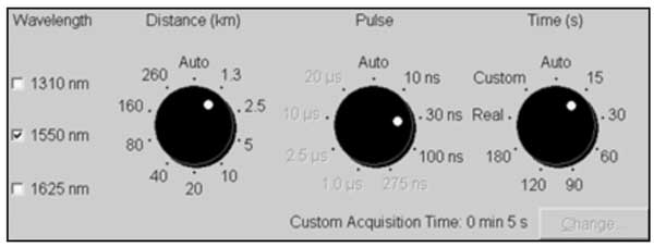
Figure 3.Main OTDR test parameters.
Distance indicates fiber length and is displayed on the screen. It is usually set greater than the length under test. Width is the duration in time (and distance) of the pulse launched into the fiber and is predetermined for specific distance ranges (e.g., shorter widths for shorter distances). For maximum resolution, select the shortest width that can reach the fiber’s end. Shorter widths can characterize events closer to the input end of the fiber and resolve two closely spaced events. Longer widths launch more energy into the fiber and reach a greater distance; however, they generate larger dead zones.
Acquisition time affects trace quality. Thousands of pulses are launched to perform a single acquisition and to average each sampling point. An OTDR removes noise from the data through an averaging process. The longer the averaging time, the less noisy the resulting trace will be.
In automated mode, the user runs the software with minimal setup. The OTDR automatically selects pulse width and distance range, optimized for the fiber under test as well as a standard acquisition time. It provides processing and output.
Interpreting results
The basic elements in a fiber profile are reflective and nonreflective events, gains and roll-offs. All the events and fiber sections located by an OTDR are listed in a result table (Figure 4), which shows the type of event, distance, loss, reflectance and attenuation.
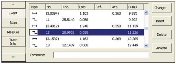
Figure 4. Data developed by an OTDR reveal details of a fiber link.
The reflective element concerns connectors, mechanical splices, breaks or the fiber end, and is recognized by a spike on the trace. The higher the spike with respect to the backscatter levels, the greater the reflectance. Nonreflective elements are caused by fusion splices or bending, which stress the fiber and cause light to escape. A discrete drop in backscatter level recognizes them.
Optical gain may occur at a splice instead of a loss; however, it is not a true increase in optical power. There are two main reasons: Optical gain is seen when backscatter level increases between the first and second fiber sections because of refractive index differences; and fiber core diameter differences cause gain from the smaller fiber to the larger fiber. True loss data for events showing gain are calculated through bidirectional trace analysis as the average between the gain and corresponding loss of the event in the reverse direction.
The end of the fiber can be viewed as a reflective or nonreflective event. An end-of-fiber condition is characterized by noise after the event. Otherwise, a backscatter level indicates a break and not the actual fiber end. A fiber end or broken fiber may not necessarily be reflective because of the nature of the end connector or break. For example, the end of the fiber can be displayed by a roll-off caused by the presence of gel or water.
Many reflective events in a fiber can cause ghost reflections, or echoes. In addition to the fiber’s reflective components, the OTDR itself may reflect light into the fiber. The light bounces back and forth within the fiber, causing false reflections at multiple distances from the true reflection. The reflections may appear within the fiber span itself or after the length of the fiber. Echoes do not exhibit losses. OTDR software can distinguish between actual events and possible echoes.
Measurement methods
An OTDR is both a troubleshooting and measurement tool. The measurement capabilities include two-point loss, end-to-end loss, splice loss, section attenuation and distance measurement.
Calculating the difference between the power levels of any two points determines the two-point loss measurement. End-to-end loss also is measured by the two-point method. Note that the end-to-end loss measurement is not as accurate as an optical loss test set measurement since the OTDR measurement is based on the reflected power and not on the actual transmitted power. Coarse attenuation loss and splice-loss measurements also can be made using the two-point method.
Splice-loss measurements are performed most accurately with the splice-loss measurement method, where loss is defined by a four-point boundary. The main markers are placed before and after the event, and the submarkers are placed beyond the main markers and do not include any additional events (Figure 5). The loss is calculated using least squares approximation.
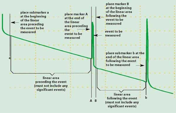
Figure 5. The splice-loss measurement method provides accurate loss information.
Attenuation measurements calculate the loss per distance based on a least squares fitting of the section. The section of fiber should not include any events within the marker limits so as not to artificially shift the line interpolation.
Distance can be measured using any of the cursor placement methods described above. When interpreting distances, the actual distance is the length of the fiber and not necessarily the cable. The fiber can be longer than the cable if it is wrapped in a helical pattern. To account for this, the index of refraction may be adjusted to scale the distance or a helix factor can be entered as an operating parameter.