Computer simulations of fiber laser designs can save thousands of dollars and weeks of time.
Dr. Mircea Hotoleanu, Dr. Per Stenius and William Willson, Liekki Corp.
From micron-size transistors to jumbo jets, all technological marvels have been simulated at some point in their development. And not only technology: Weather, stock markets and even the future of human society are predicted by computers — although the last, so far, is available only in Isaac Asimov’s novels. For that reason, we are not going to explain what a computer simulator is and how it helps to design more quickly, more accurately and less expensively. The purpose of this article is to present what makes an accurate and reliable fiber laser simulator and how to use it in product design, engineering and manufacturing. Including examples of real applications, this article unveils the dos and don’ts of simulating a fiber laser.
In 1996, we attended a workshop in Porto, Portugal, where the main subject was the future of fiber lasers. Many papers with optimistic or pessimistic views were put on the table. Although telecom was booming, the subject of fiber lasers was left in a shadow for a while. However, 10 years later, the fiber laser has become the most dynamic sector of the laser business, with an annual growth rate of more than 50 percent. And although most of the market belongs to only a few fiber laser manufacturers, the potential of the devices is far from exhausted.
For that reason, tens of other companies, large and small, invest a lot of time and money in research and development of fiber lasers, subsystems, components and fibers.
The road to bringing a fiber laser to the market is long and snaky and has many hurdles. However, the potential and advantages of this device in comparison with “traditional” lasers more than compensate for the risks. The all-too-familiar scenario presented in the prologue is just one source of delays and high costs that may be reduced by simulations.
A good simulator
Depending on the operating conditions, there are many possible designs for a fiber laser. Two of the most common are presented in Figure 1: CW lasers and MOPA (master oscillator power amplifier) systems, which generate light pulses. A CW fiber laser usually consists of an active fiber spliced between two fiber Bragg gratings (reflectors) and a pump laser. A MOPA system is built using a low-power pulsed signal source (usually called “seed”) that is fed into a power amplifier.
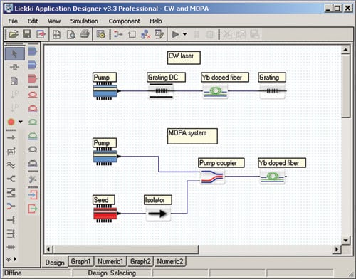
Figure 1. Two fundamental fiber laser configurations are shown. These configurations, and all imaginable variations, can be simulated by dragging individual components from the “parts box” on the left of the screen into the main screen.
Software that simulates such designs should implement the mathematical models of all components and should have an algorithm for calculating the optical power propagation in between components. Such simulators have been in use for many years, especially for telecom applications. Both homemade programs and commercial products have helped telecom laboratories and companies reduce the time to market of new fibers and erbium-doped fiber amplifiers.
Are these simulators useful for high-power fiber lasers? The answer is an emphatic no. There are at least two main reasons for that: The optical fibers used in fiber lasers are much more complex than those used for telecom applications, and they usually work in very different power, wavelength and thermal regimes. For instance, whereas the erbium-doped fiber for a telecom amplifier usually works up to several hundred milliwatts at 1525 to 1610 nm and has a maximum operating temperature of 40 to 50 °C, in a high-power fiber laser the doped fiber handles hundreds of watts at 1060 to 1115 nm and a top operating temperature close to 100 °C.
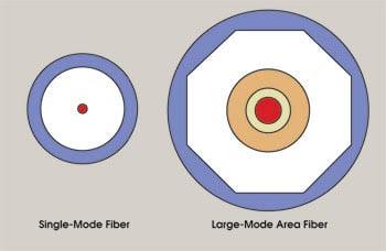
Figure 2. The fibers used for fiber lasers are much more complicated than those used in standard telecom applications.
The physical differences between standard telecom optical fibers and the fibers used for high-power fiber lasers are evident in Figure 2. The telecom fibers have a small core size (usually between 2 and 10 μm) that guides a single propagation mode. For that reason these fibers are referred to as single-mode fibers (SMFs). To handle high-power beams, fibers for lasers have much larger core diameters (as large as 100 μm), and they are referred to as large-mode-area (LMA) fibers.
LMA fibers usually work in the multimode regime (more than one mode is guided). However, because users quite often like to obtain a single-mode output from an LMA fiber, the fiber either is coiled or its refractive index and/or dopant profiles are tailored. A good fiber laser simulator must be able to model all of these characteristics.
However, there are some other important differences. Single-mode fibers usually guide light in the core only, whereas LMA fibers have a special coating that allows the light to be confined also in the cladding around the core. This structure is called a double-clad fiber.
Because of the high power density, the fibers used in fiber lasers are quite often working close to the threshold for nonlinear effects, which can be deleterious because they drain power from the laser signal. To keep the system below the threshold of nonlinear effects, the fibers should be as short as possible. That implies high rare-earth concentration in the core. Thus, the fiber laser simulator must be able to model high dopant concentration effects (for instance, clustering) and to evaluate the nonlinear thresholds.
All these fiber characteristics require more complex models for LMA fibers than those used for single-mode fibers. In addition, there are even more differences to be considered. The vast majority of applications using active single-mode fibers are amplifiers or amplified spontaneous emission sources. In these systems, the reflections, although sometimes relevant, do not play a fundamental role. For a laser, obviously, the reflections are essential, and, thus, a fiber laser simulator must accurately model any reflection that is generated within the system.
Although accurate fiber modeling is crucial, it is not enough. We mentioned the necessity of having a proper evaluation of the power transmission between optical components. In addition, there are several other tools useful in determining design, engineering and manufacturability, such as optimization tools and Monte Carlo analysis. All this functionality will place a heavy burden on the computer running it. For that reason, the calculation algorithms must be not only accurate and robust but also fast.
A final word on one of the qualities that a fiber simulator must possess: It must be easy to use. Complicated models, algorithms and sophisticated optimizations might lead quite easily into a “forestlike” interface with countless buttons and menus. An ideal simulator should allow the user to focus on the physics of the laser system to be designed and not on the software manuals.
Using a simulator
Assume that you have an ideal fiber laser simulator. How do you use it to the best advantage? Whether you are a student learning the basics of active fibers, a fiber laser designer, a manufacturing engineer seeking the highest yields, or a user of the fiber laser or amplifier, simulation always can help you in your activity.
Because it is in an early stage of development, the fiber laser industry still is evaluating numerous fiber designs. Various core compositions, sizes and shapes are tested to enhance the fiber gain and beam quality and to reduce noise and nonlinearities. Various cladding sizes, shapes and coating materials are used to allow the coupling and distribution of higher pump power. Depending on the manufacturing technology, it can take from two days to two weeks to produce a new fiber, and it might cost thousands or tens of thousands of dollars. Then follows the testing, and — usually after a month — the cycle restarts to improve a successful design, or simply to start over if the design was unsuccessful.
A good fiber laser simulator often can reduce this month(s)-long cycle to hours. The fiber designer can optimize all of the parameters before fabricating the fiber, the system designer can choose the right layout and components to optimize the performance, and the manufacturing engineer can evaluate the acceptable tolerances and the production yield. Moreover, when the finished product is shipped, the end user can predict its behavior in various working conditions.

A good fiber laser simulator allows the user to adjust as many component parameters — as well as system parameters — as possible. For instance, the active fibers must be described by glass dimensions, refractive index and doping concentration profiles, emission and absorption cross sections, nonlinear coefficients, cluster concentration, and, of course, length and bending radius. For the passive components (such as isolators, filters and splices), there should be an adequate list of parameters, from which the return loss should definitely not be excluded, because the simulator must be able to describe the effect of any resonators. All of these parameters must be available at the time of simulation.
A simulator uses complicated algorithms to describe the optical performance. Usually, the user sets the acceptable levels for absolute or relative errors in finding the solutions of these equations. These levels define the calculation accuracy. There is a trade-off between the calculation accuracy and the computer time required for the calculation: The better the accuracy, the longer the calculation time. For that reason, common sense should be used in setting the accuracy level, based on the expected level of optical powers in the system.
For example, it is reasonable to set the accuracy to 1 mW if the laser produces milliwatts. However, for a kilowatt laser, a 1-mW accuracy requirement will increase the calculation time unnecessarily. On the other hand, if the accuracy is too lax, the results might be unreliable. You can check this situation when browsing the simulation results. If you find an optical beam having a power lower than the accepted absolute error, the result is unreliable, and you should increase the calculation accuracy.
Obviously, the main purpose of the simulation is to generate results that predict the behavior of the real system. Thus, the quality of a simulator is measured by comparing the simulated data with the measured data. Although this is reasonable — and, in practice, the ultimate test — one should not overlook the possibility that both simulation and measurement might be affected by errors. We list here several elements that should be considered when making this comparison:
• The models have a certain domain of applicability — a domain where the errors can be estimated relatively precisely and can be controlled. When the system works outside this domain, the simulation results could be erroneous or unpredictable.
• The models use parameters that have been measured previously. Any error in that measurement will adversely affect the simulation result. For instance, the accuracy of the active fiber emission and absorption cross sections is crucial for the accuracy of the result. As with any simulation, the GIGO (garbage in, garbage out) principle applies.
• Some models have a large degree of uncertainty because the real components may have large distributions of values for their parameters. For example, the splice loss between optical fibers is an unpredictable value within some confidence range and, in most cases, impossible to measure accurately. To cope with such situations, a Monte Carlo analysis can be used to predict the spread of the results when some parameters are randomly distributed inside the confidence range.
• Sometimes in the simulation process, human interaction might, intentionally or not, affect the accuracy. In some cases, the user makes some simplifications in the design, hoping that it will have an effect on the result that is minimal or easy to evaluate. This requires a lot of experience.
However, an “I know what I am doing” attitude is responsible for big errors in many cases. For instance, if the user tries to increase the simulation speed of an erbium-doped fiber amplifier by removing an isolator from the design, the results may be significantly affected both in the amplified spontaneous emission spectral shape and in the signal power. In other cases, the user is not aware of some component properties or misses the component entirely.
• The settings of the measurement equipment may introduce significant deviations from the “real” value. For example, if the 976-nm peak absorption of an ytterbium-doped fiber is measured with a spectrum analyzer having 1-nm spectral resolution, the measured value might be 30 to 50 percent lower than the real value.
• The measurement equipment may affect the measured system, thus producing erroneous results. For instance, any backreflections into the laser from the measuring equipment can dramatically alter the performance of the laser.
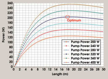
Figure 3. These sample curves show how a simulation can help the laser designer select the optimal length of fiber to obtain a 200-W output from minimal pump power. The ideal design requires 18 m of fiber.
The most common application of a fiber laser simulator is to evaluate the optimum active fiber length and pump power level. As displayed in Figure 3, from a simple iterated simulation one can find both optimal values. This is but one example of situations where simulation can save time and money.
When the CW laser in Figure 1 is initially turned on, it can produce a high-power transient pulse that might damage both the fiber and the pump source. The simulator can predict this behavior and show how adjusting the pump rise time can reduce it (Figure 4).
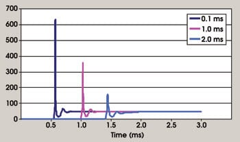
Figure 4. The switch-on transient can be reduced bylengthening the pump rise time from 0.1 to 2.0 ms.
Many fiber lasers depend on bending losses to discourage propagation of high-order modes. However, bending the fiber also introduces mode-field deformation, and this effect must be taken into account by the simulation (Figure 5).
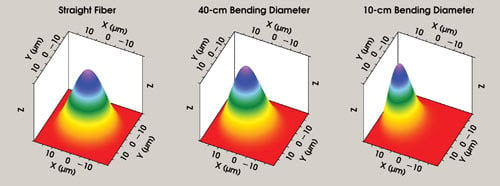
Figure 5. Bending the fiber to increase the propagation loss of high-order modes also introduces mode-field deformation. Shown here is the simulation’s prediction of the deformation for different bending radii.
The yield is an important parameter for evaluating the manufacturability of the fiber laser. A simulator that has implemented a Monte Carlo algorithm can provide yield evaluation based on the tolerances of the components and procedures used in the manufacturing process (Figure 6).

Figure 6. The manufacturing yield can be evaluated with a Monte Carlo analysis, based on the tolerances of components used.
You may imagine countless other applications for a fiber simulator. It is not just a tool to cut costs and increase efficiency; more importantly, it lets one inexpensively explore those seemingly unlikely solutions that could evolve into the next quantum leap in laser performance.
Meet the authors
Mircea Hotoleanu is the product manager for design software at Liekki Corp. in Lohja, Finland. He leads the development team for Liekki Application Designer fiber laser simulation software; e-mail: [email protected].
Per Stenius is the CEO of Liekki Corp.; e-mail: [email protected].
William Willson is president of Liekki Inc. in the US and vice president of sales and marketing of Liekki Corp.; e-mail: [email protected].