Two-color fluorescence-based methods are uncovering molecular interactions inside cells. A guide to measuring colocalization ensures that these techniques work.
Jonathan W. D. Comeau, Santiago Costantino and Paul W. Wiseman, McGill University
Intermolecular interactions between receptors and small ligands, nucleic acids and proteins, as well as between various proteins, are tightly regulated within cells as the molecular-level mechanism that controls almost all biochemical processes — including enzymatic catalysis, growth, signaling, migration, transcription and translation.
The identification of particular molecular interactions therefore has been a crucial first step in many cellular studies. Traditionally, biochemical techniques have proven to be an effective indicator of interactions between two proteins of interest. These techniques are almost always limited to in vitro studies, however. More recently, technological advances in fluorescence microscopy and fluorescent protein labeling have opened the door to a wide variety of in vivo protein interaction studies.
Combined with relatively simple image analysis tools, developments in fluorescence microscopy have helped reveal a number of newly discovered interactions in cells. Researchers take advantage of new methods not only for the simple detection of interactions within cells, but also to quantify the fraction of protein (or other molecule of interest) that is participating in the interactions.
Of course, as with any quantitative analysis, meaningful results are obtained only after a thorough characterization of the capabilities and limitations of a particular technique. Thus, a recent detailed investigation of the accuracy and precision of various image colocalization analysis techniques served to validate one of the new crop of fluorescence-based methods: measuring interactions in cells via analysis of two-color fluorescence microscopy images.
Obtaining accurate results
With this technique, the two molecules of interest are labeled with distinct fluorophores, and the cells are imaged using either confocal, two-photon or total internal reflectance fluorescence microscopy, with spectrally separated image acquisition in two detection channels. Interactions typically are measured by evaluating the amount of signal colocalization present between the two images.
In this context, colocalization is simply the fraction of labeled molecules that is present in the same locations in each image pair, as determined by the spatial overlap of the pixel intensities in the two images. It is considered an indirect measure of interaction, however, as some pairs of molecules end up in close proximity simply by chance. Exacerbating this is the fact that the optical resolution limit is more than an order of magnitude larger than molecular dimensions. Still, the statistical nature of the calculations ensures that colocalization is a strong predictor of molecular interactions, as long as sampling is sufficient.
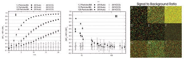
Errors in the measured interaction fraction (M1) may be a function of the counting noise width factor, a measure of the broadening of the fluorescence intensity Poisson distribution, which typically increases as the detector gain is increased, or a function of the signal-to-background ratio. Example images are shown here. Background noise was added to the images in the second row and counting noise to the images in the third row. BA = beam area. Reprinted with permission of Biophysical Journal.
Originally reported in 1993, the Manders’ colocalization coefficients — M1 and M2 — have become ubiquitous measures of the amount of colocalization present in two-color fluorescence microscopy images and now are standard issue in many recent commercial image analysis software packages.1
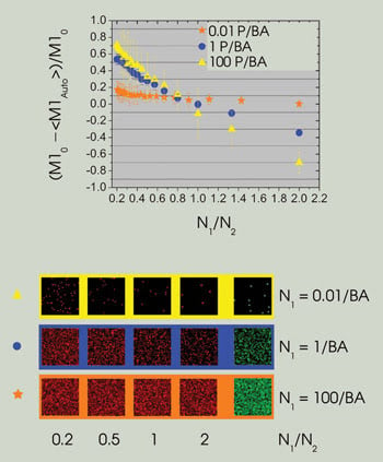
The dependence of the error in colocalization analyses on the density ratio between channels is a function of total density. At very low densities [0.01 particles per beam area (P/BA)], the error is relatively constant as a function of the density ratio. As the density increases, however, the slope of the line increases dramatically, leading to large errors in automatic colocalization. Example images for three density ranges plotted are shown in the bottom panel. (M10 refers to the simulation input value. Graphs reprinted with permission of Biophysical Journal).
The colocalization coefficients are calculated by finding the intensity-weighted ratio of all colocalized pixels to the total number of pixels in each detection channel (M1 or M2). The set of colocalized pixels is defined by accurate localization of the pixel pairs above a particular intensity threshold, which is essential to the correct evaluation of M1 and M2. To remove ambiguities in the manual determination of this intensity threshold, researchers reported an automatic threshold determination method, referred to as automatic colocalization, in 2004.2
Spatial image cross-correlation spectroscopy (ICCS) is a lesser-known technique used for colocalization analysis.3,4 In ICCS, intensity fluctuations within the pixels of one image channel are spatially cross-correlated with the corresponding pixels of the other, yielding what is referred to as the zero spatial lags correlation value. The second image is subsequently shifted by one pixel withrespect to the first, and the shifted pixels are then correlated.
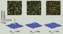
In image cross-correlation spectroscopy (ICCS), intensity fluctuations within the pixels of one image are spatially cross-correlated with the corresponding pixels of the other image. This gives rise to a cross-correlation function whose shape is related to the point spread function of the microscope, and the amplitude of which is directly proportional to the number of interacting particles. Detection limits in ICCS arise from the background correlation between randomly overlapping pixels. This effect is illustrated by the decreasing correlation function amplitude as the amount of interacting (colocalized) particles in the images decreases. The corresponding overlaid images are shown above (one particle per beam area ).
This shifting procedure is continued until all possible spatial lags have been calculated in X and Y, producing a two-dimensional cross-correlation function with a profile identical to that of the point spread function. The amplitude (zero spatial lags value) of the resulting spatial cross-correlation function is directly proportional to the number of interacting particles that are present in the system.
ICCS, therefore, provides not only the fraction of interacting particles but the absolute-number density as well. The amplitude of the spatial cross-correlation function usually is estimated from a nonlinear least squares fitting of a Gaussian function to the correlation data.
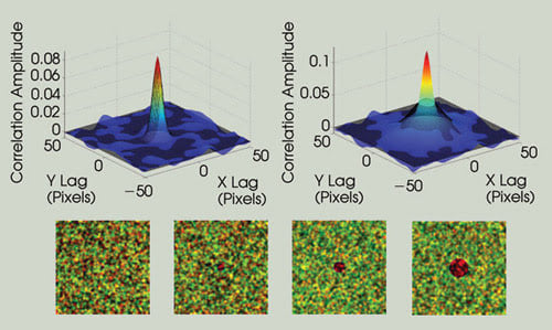
Spatially nonuniform particle distributions perturb the ICCS measurement. This is illustrated by adding an increasingly large “hole” in the center of one of the image channels. As the perturbation becomes larger, the autocorrelation function for that channel deviates from the ideal point spread function shape (much larger radius), which eliminates the possibility of performing the fitting routine necessary for ICCS measurements. The correlation functions are shown in solid color, and the Gaussian fits are shown as a black mesh.
Given the statistical nature of ICCS, precise results are obtained when a large number of fluctuations are sampled within an image area. This occurs when the ratio of the image area to the focused laser beam area — which sets the size of a sampled spatial intensity fluctuation — is large.
Obtaining accurate results requires understanding the various sources of error and then minimizing or correcting them in any measurement of colocalization, regardless of the technique employed.
Sources of error include the detection of fluorescence from the green-shifted dye in the red-shifted detection channel (cross-talk), detection of fluorescence inherently present in the cell (autofluorescence), nonspecific labeling of the species of interest and photon detection noise. Researchers can greatly reduce or completely eliminate any of these vexing issues with experimental control.
One very important factor cannot be controlled readily, however: the intrinsic molecular or particle density within the cellular system. The particle density sets detection limits and, therefore, should be of primary concern when attempting a colocalization measurement.
For this reason, we focused on this factor in a recently published guide to accurate fluorescence microscopy colocalization measurements. To address the effect of particle density in many different experimental situations, we analyzed hundreds of simulated images with the two methods described above and evaluated the error in the measured colocalization.
Measuring colocalization
The first step in measuring colocalization is to consider the detection limits one might expect for the two colocalization techniques. In principle, automatic colocalization can accurately detect colocalization for as little as 3 percent of interacting molecules. The detection limit in ICCS depends on random overlap, on the fitting procedure and on the overall particle density of the system. As the interaction fraction decreases, the central peak in the correlation function proportional to the number of interacting particles decreases, and is eventually masked by the background correlations from randomly overlapping particles. This process leads to detection limits between 15 and 20 percent (M) interaction for images of 256 × 256 pixels.
The effect of higher densities on colocalization measurements is illustrated by fixing the number of interacting particles in the first image while varying the particle density in the second. Very large errors in the automatic colocalization method become evident as the densities within the two images diverge. In fact, the relative error in the channel 1 interaction fraction (M1AUTO) was found to be almost 80 percent when the particle densities differed by only a factor of two between images.
This effect is more pronounced at larger particle densities (one to 100 particles per beam area) — implying that, if the density of the system were at all elevated, both species must be present in approximately equal numbers to obtain accurate results with this method.
It is also worth noting that verifying the results of this type of measurement is almost impossible after the fact. For this reason, having some prior knowledge of the system is particularly important when using this colocalization method.
ICCS is much less affected by differences in the density ratio between the images than is automatic colocalization. The relative error in the ICCS analyses was less than 10 percent as long as the particle density ratio was less than 10; the fitting of the correlation function generally fails for larger ratios. This remains true even as the total particle density rises. Thus, ICCS will provide accurate colocalization results for density ratios of 10 or lower. Moreover, it includes a built-in check not available with automatic colocalization because the fitting fails outside of this range.
The uncertainty associated with photon emission and detection is an important consideration in any measurement based on light detection. This type of noise is governed by a Poisson distribution that is typically broadened as the detector gain increases in conventional systems with analog detectors.
Defining a parameter called the width factor — a measure of this broadening phenomenon — made it possible to measure the effects of increased detector gain on the error in colocalization measurements.
Once again, the particle density plays an important role in determining the resulting error obtained via automatic colocalization analysis. The largest errors occur when the width factor is high (high detector gain) and the particle densities are also high (10 to 100 particles per beam area). Using ICCS reduces these errors significantly.
The amount of interaction in ICCS is determined by taking the ratio of the densities of the interacting species to the total number of species for a given channel. If the noise levels of the two detectors are approximately equal, then the errors in the measured interacting and noninteracting densities essentially cancel each other out. In automatic colocalization, real experimental width factor values will lead to significant errors, depending on the particle densities.
More systematic sources of noise — such as dark current, autofluorescence and scattered light — can, in most cases, be accounted for by a simple global intensity subtraction. At the very least, this type of correction must be performed before any colocalization analysis is applied to the images in question. A signal-to-background ratio can be defined as a measure of this type of noise using the average maximum of the fluorescence intensity signal and the standard deviation of the residual noise remaining after correction. Low signal-to-background ratios will lead to large errors in automatic colocalization analyses, although proper image correction will normally result in reasonable ratios and accurate measurement of colocalization.
Another important consideration for ICCS is the spatial distribution of particles within the images. Nonuniform particle distributions in space — heterogeneous structures or edge boundaries where the fluorescence intensity drops off (or increases) rapidly — will perturb the fitting of the correlation function. In certain cases, this problem can be mitigated by selecting an alternate region of analysis. In addition, information regarding the actual pixel locations of the interacting particles is lost in ICCS because of the spatial averaging that is performed across the area analyzed. On the other hand, the automatic colocalization technique is not affected by image inhomogeneities and does define the locations of the colocalized pixels.
Taken together, automatic colocalization and ICCS provide a large dynamic range for accurate measurements within fluorescence microscopy images. Our study demonstrated that the intrinsic variable of particle density, which is often overlooked, must be carefully considered when measuring colocalization.
We have identified four key experimental guidelines for choosing an appropriate colocalization method and obtaining accurate results: (1) If possible, estimate the expression densities of the species of interest. (2) Acquire two-color images by optimizing detector gain levels (and laser powers) to have a large signal (without saturation) but minimal noise. (3) Evaluate noise levels present in the images and perform any necessary corrections. (4) Evaluate the particle distribution within the images.
Meet the authors
Jonathan W. D. Comeau is a Ph.D. student in the department of chemistry at McGill University in Montreal; e-mail: [email protected].
Santiago Costantino is a postdoctoral fellow in the department of physics at McGill University; e-mail: [email protected].
Paul W. Wiseman is an assistant professor in the departments of physics and chemistry at McGill University; e-mail: [email protected].
References
1. E. Manders et al (1993). Measurement of co-localization of objects in dual color confocal images. J MICROSC, Vol. 169, pp. 375-382.
2. S. Costes et al (2004). Automatic and quantitative measurement of protein-protein colocalization in live cells. BIOPHYS J, Vol. 86, pp. 3993-4003.
3. S. Costantino et al (2005). Accuracy and dynamic range of image correlation and cross-correlation spectroscopy. BIOPHYS J, Vol. 89, pp. 1251-1260.
4. J. Comeau et al (2006). A guide to accurate fluorescence microscopy colocalization measurements. BIOPHYS J, Vol. 91, pp. 4611-4622.