Ruisheng Lin, Alex Clowsley, Isuru Jayasinghe and Christian Soeller, Biomedical Physics, University of Exeter
EMCCD-based cameras with high quantum efficiencies and low readout noise characteristics traditionally have been the preferred technology for SMLM superresolution imaging. However, with tailored localization algorithms, sCMOS cameras have become a notable alternative for superresolution microscopy.
The ability of optical superresolution microscopy to circumvent the so-called “diffraction limit” has revolutionized the use of fluorescence microscopy to study subcellular and molecular-scale biological processes. Single-molecule localization microscopy (SMLM) – also commonly referred to as PALM, STORM and dSTORM, among other acronyms – overcomes the resolution limit by measuring the position of large numbers of marker molecules and can achieve effective lateral detail resolution in excess of 20 nm1–4 in addition to similar improvements in axial resolution.
Typically, to reconstruct a single 2-D or 3-D image, several thousand camera frames have to be acquired and analyzed.5 Preferred camera technologies combine the ability to sustain high frame rates with the capability to detect the comparatively low light levels associated with single- molecule fluorescence emission. Such cameras should enable the rapid image generation that often is required for live-cell recordings.
Traditionally, electron multiplying CCDs (EMCCDs) have served as the dominant technology within this realm. EMCCDs are widely used in superresolution imaging because the best back-thinned EMCCDs combine high quantum efficiency with very low readout noise.
In the consumer market for digital cameras, CMOS-based sensors effectively have replaced CCD sensors due to lower manufacturing costs and considerable improvements in CMOS sensor technology. For example, CMOS-based DSLR cameras are now widely used by hobbyists for light-sensitive tasks like astrophotography. Research-grade CMOS cameras, sometimes branded as scientific CMOS or sCMOS cameras, have become available from several manufacturers. These cameras are capable of recording at high frame rates (approaching 1000 frames per second in reasonably sized regions of interest) and have low readout noise, peak quantum efficiencies up to about 70 percent, and provide megapixel densities and high dynamic ranges.6–10 In addition, the cost of CMOS cameras typically is a fraction of that of EMCCDs, which makes CMOS cameras an attractive alternative for single-molecule-based superresolution imaging.
One potential drawback of CMOS cameras is their pixel-dependent sensor characteristics. Unlike EMCCDs, where all photoelectrons are converted and amplified through a common readout structure, CMOS cameras’ pixels each have their own readout and processing electronics. Therefore key properties like readout noise, offset and sensitivity of CMOS cameras are not uniform throughout the entire sensor area.11,12
In SMLM, each raw data frame contains images of a subset of the whole population of marker molecules, and a series of frames is used to collect the positions of a large percentage of the marker population. In the simplest implementation, the fluorescence-emitting molecules in a single frame are sparse enough so that their images do not overlap, allowing their positions to be measured with high precision. Localizing marker positions is typically achieved by fitting a model to the data to determine the central coordinates of each blink.13,14 An efficient and comparatively simple approach uses a Gaussian model for rapid 2-D localization, and more complex models can be used for full 3-D localization in conjunction with point spread function engineering. Unfortunately, the pixel-dependent characteristic in CMOS cameras makes using the conventional algorithms – which assume uniform pixel properties and work well with EMCCD cameras – problematic, because local pixel property variations introduce bias and therefore may not reliably determine the position of each molecule.15–17
The bias resulting from pixel nonuniformities can be eliminated by employing localization algorithms that explicitly take into account the camera-specific pixel properties. These algorithms use information on the nonuniform noise characteristics, offsets and sensitivity to determine an unbiased position estimate. It has been shown that if CMOS cameras are provided with suitable algorithms, these cameras can achieve highly precise localization and achieve performance that rivals that of EMCCDs – all while allowing for a larger field of view and fast frame rates.7
We sought to implement a simple, unbiased algorithm for 2-D position determination in SMLM, the goal of which was to evaluate whether current CMOS cameras are a viable alternative to EMCCDs, while still preserving the simplicity of the software interface that we currently use.
Setup and data acquisition
A simplified schematic of an SMLM system, such as the one in our laboratory that uses both an EMCCD and a CMOS camera, is shown in Figure 1a. Acquisition is controlled using our Python-based PYthon Microscopy Environment (PYME), which can be obtained at the Bitbucket code repository. PYME offers a data acquisition module that performs microscope and camera control and is optimized for PALM-/STORM-type superresolution imaging. Customizable acquisition protocols allow users to predefine a series of hardware setting changes (e.g., beam intensity or camera settings) at defined times during the acquisition process while providing CPU-parallel, real-time analysis. In short, PYME seamlessly integrates the Python programming language with a robust combination of powerful features for microscopy.
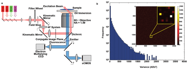
Figure 1. (a) Simplified schematic of a custom-built STORM microscope system. Beams from several laser modules are coupled and propagate through a neutral-density filter wheel. A field stop is used to adjust the area of illumination in the sample. A 4F optical system is inserted with its back focal plane coplanar with the conjugate plane of the sample plane, and the two mirrors in the system are mounted in kinematic holders, allowing the illumination position and beam angle to be adjusted. Images are recorded using either an EMCCD or a sCMOS camera. (b) Maps and histograms of the pixel-dependent noise variance in the full region (2048 × 2048) of an Andor Zyla 4.2 sCMOS camera. The variance ranges from <1 to 2500 ADU2 (analog-to-digital units squared), indicating nonuniform noise characteristics of the sensor chip.
We evaluated the performance of a Zyla 4.2 CMOS camera (10 Tap connection). An Andor Ixon Ultra EMCCD served as the reference. Both cameras were controlled via manufacturer software development kits (SDKs), which were used in custom back-end implementations within our PYME environment.
Determination of camera properties
The Zyla CMOS camera offers two real-time filters that ensure more visually appealing images by filtering out “spurious noise” and applying “static blemish correction.” During data acquisition for superresolution imaging, these filters should be disabled. Offset, dark current and read noise can be measured by recording a series of dark frames. Offset and total temporal noise (i.e., read noise plus dark current contributions) are measured as the mean and standard deviation of the frame series, respectively, and are determined on a pixel-by-pixel basis. The dark current is proportional to the integration time and can be obtained by employing a linear regression on data obtained with different camera integration times. In practice, given the short integration times used for SMLM, determining the total temporal noise was sufficient. The extent of the variability in read noise between pixels is illustrated in the color-coded map (Figure 1a), and the frequency histogram of the measured temporal noise variance is shown in Figure 1b.
To determine sensitivity variation, the gain can be measured via a photon transfer curve on a pixel-by-pixel basis.7 Alternatively, we estimated the photon response uniformity by imaging a smooth input signal (e.g., a heavily defocused fluorescein droplet) followed by 2-D Gaussian filtering of the offset subtracted mean signal. In response, the smoothing filter locally flattens the variation; the variation then can be obtained by comparing raw offset corrected mean with smoothed mean. In our experiments, the variations were relatively small and did not have a strong influence on the model fitting process.
Most important for the user, the determination of pixel-specific camera maps essentially is a one-off procedure, and processed camera maps can be stored for all future SMLM analyses. Some care may have to be taken during the characterization procedure to match the gain settings and other adjustable camera parameters to those typically used for SMLM acquisition.
CMOS localization algorithm
In our implementation, all pixel properties are predetermined and available as camera maps that indicate offset, read noise and pixel sensitivity, all of which are handled by a user-defined class in Python that is provided to the algorithm during real-time analysis. The raw data from the camera first is corrected by removing local pixel offsets and applying pixel sensitivity corrections; photoelectron conversion also is implemented at this stage. We fit a 2-D Gaussian model with a background using a weighted least squares (WLS) algorithm. The weight given to each pixel is inversely proportional to the total noise variance in each pixel, which is estimated as the combination of read noise (Figure 1b) and Poisson shot noise, the variance of which is estimated from the pixel photoelectron count. As a result, high-noise pixels have a smaller weight and contribute less to the localization process. Thresholds can be chosen to exclude pixels from fitting completely, which is achieved by assigning an artificially high read noise to them (e.g., 106), thereby making their contribution negligible. The parameters that minimize the WLS fit are recorded and include center locations, amplitude, image width and background. The covariance matrix returned from the least squares fit routine is used to estimate confidence intervals for all parameters.
It has been noted that the WLS problem can become unstable under certain conditions but is well-behaved in the presence of non-negligible backgrounds, which we typically find is the case in SMLM experiments with biomedical samples – and exceptions are detected by our implementation. Overall, the simplicity of the algorithm, its rapid convergence using a Levenberg-Marquardt routine and its well-understood behavior make it very suitable for SMLM.
Validation with subresolution beads
We validated the algorithm using an image series (~4000 frames) of 100-nm Ø beads recorded with low-intensity illumination and high frame rate (100 fps).
The average number of photons in each event was approximately 900 – close to the photon yield of commonly used fluorochromes. Both the conventional as well as the new CMOS algorithm were used to determine bead locations; the same drift correction was applied in the data analysis process. The localization results were rendered into a 2-D position map by a quad-tree-based adaptive histogram method (Figure 2).18 The comparison clearly shows the distortion in the cloud of localizations resulting from the uncorrected bias using the conventional algorithm. It also shows an estimated 22 percent improvement to the localization precision with the use of the camera-specific maps.
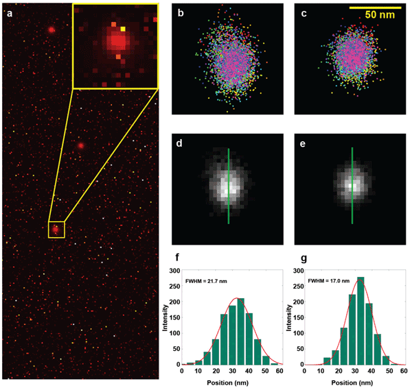
Figure 2. Comparison of the localization results from the conventional and new algorithms. (a) Temporal variance of an image series of fluorescent beads (0.2-μm orange-red fluospheres) reveals the noisy pixels and their presence relative to bead locations, which are seen clearly due to the shot noise properties of bead signals (see inset). (b) and (c) Localization results from the conventional and new algorithm. Bias is introduced by the presence of noisy pixels. Note the correlation between the spread direction in b and the high-variance pixels in the inset in a. The bias is essentially eliminated by our algorithm c. (d) and (e) Reconstructed images generated from the localization results in b and c. (f) and (g) The profiles of the green lines in d and e illustrate a 22 percent (measured as full width at half maximum of 17.0 nm versus 21.7 nm) improvement of the localization uncertainty, resulting in better localization precision and the absence of bias.
Qualitative comparison with EMCCD data
Although the quantum efficiency of EMCCDs is higher than that of our CMOS camera (90 percent vs. 50–70 percent, respectively), the additional noise that is generated during the electron amplification process in the EMCCD effectively reduces the signal-to-noise ratio by a factor of √2, equivalent to reducing the effective photon count by half. In essence, this halves EMCCDs’ effective quantum efficiency and makes it comparable to that of the CMOS camera. We qualitatively compared both the signals and the locations of the beads by switching between cameras and concluded that the CMOS data was at least comparable to data obtained from EMCCDs for localizations. In most cases, though, the data indicated slight improvements of CMOS-based localizations versus those of our EMCCD-based localizations.
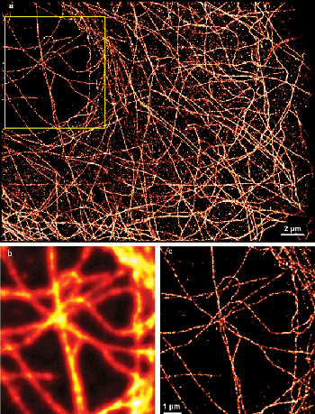
Figure 3. Superresolution image of microtubules in COS-7 cells labeled with Alexa 680. (a) The entire 30 × 40 μm2 region of interest. The corresponding (b) diffraction-limited and (c) superresolution images of the boxed region. A significant improvement of resolution reveals more detail of the microtubule structure.
Imaging biological samples with a CMOS camera
We now regularly use the Zyla CMOS camera for SMLM and show some typical results as illustration. Figure 3 shows a superresolution image of microtubules in COS-7 cells labeled with secondary antibodies conjugated to Alexa 680. Compared with the blurred, diffraction-limited image, the superresolution image clearly shows the details of the microtubular network. Additionally, although the 30 × 40-μm2 region of interest uses only about 5 percent of the camera’s active pixel area (equivalent to 148 × 148 μm2 in the sample, typically large enough to image a multitude of cells), it would almost cover the entire pixel area of an EMCCD camera. We rarely use the full size of the detector for SMLM, as we can cover sufficiently large sample areas using a subset of pixels. In addition, the relatively high laser intensities required for STORM limit the size of the illuminated field, and large ROIs impose high CPU demands on real-time analysis. Accordingly, most users will be able to choose a more affordable, USB-based connection option for a CMOS camera (if available) that is able to support maximal frame rates for reasonably sized ROIs. In our experience, the large pixel count of CMOS sensors is useful when identifying areas of the sample for SMLM imaging, as the chip size allows for covering a comparatively large field of view – typically much larger than that covered by EMCCDs.
Another example is the superresolution image of small membrane structures in equine heart cells, called transverse tubules, which are shown in Figure 4 and are stained by the membrane marker WGA Alexa 680. A significant improvement in resolution is achieved and details of the complex membrane topologies are revealed in the superresolution image.
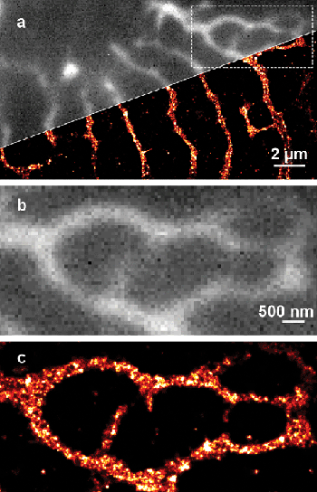
Figure 4. A 10-µm-thick section of equine ventricular cardiac muscle labeled using wheat germ agglutinin (WGA), conjugated to Alexa Fluor 680, reveals the cell membrane and T-tubule network. (a) Superresolution image of a small area in the tissue sample; note the improved resolution as compared to the conventional wide-field region. (b) The corresponding wide-field and (c) superresolution images of the boxed region. The improvement in resolution reveals finer tubules and the detailed shape of wider tubules.
In conclusion, modern sCMOS cameras provide a formidable option for superresolution imaging. The advantages of fast data acquisition, large field of view and reasonably high effective quantum efficiency make it an attractive choice. With tailored algorithms, the apparent disadvantages (compared to those of EMCCDs) can be fully compensated. In the near future, we aim to fully integrate camera-specific algorithms into the PYME suite so that the microscope operator can seamlessly benefit from algorithmic improvements. The combination of ongoing advances in hardware and software technologies should help to further pave the way for routine and straightforward superresolution imaging.
Meet the authors
Dr. Ruisheng Lin is an associate research fellow at the University of Exeter, UK; email: [email protected]. Alex Clowsley is a PhD student at the University of Exeter, UK; email: [email protected]. Dr. Isuru Jayasinghe is an associate research fellow at the University of Exeter, UK; email: [email protected]. Professor Christian Soeller heads the Laboratory for Biophysics and Biophotonics in the Biomedical Physics Group at the University of Exeter, UK; email: [email protected].
References
1. E. Betzig et al (2006). Imaging intracellular fluorescent proteins at nanometer resolution. Science, Vol. 313, pp. 1642-1645.
2. T.J. Gould et al (2012). Optical nanoscopy: from acquisition to analysis. Annu Rev Biomed Eng, Vol. 14, pp. 231-254.
3. S.W. Hell (2009). Microscopy and its focal switch. Nat Methods, Vol. 6, pp. 24-32.
4. S. van de Linde et al (2012). Live-cell superresolution imaging with synthetic fluorophores. Annu Rev Phys Chem, Vol. 63, pp. 519-540.
5. M.J. Rust et al (2006). Subdiffraction-limit imaging by stochastic optical reconstruction microscopy (STORM). Nat Methods, Vol. 3, pp. 793-795.
6. H.T. Beier and B.L. Ibey (2014). Experimental comparison of the high-speed imaging performance of an EM-CCD and sCMOS camera in a dynamic live-cell imaging test case. PLOS ONE, Vol. 9, p. e84614.
7. F. Huang et al (2013). Video-rate nanoscopy using sCMOS camera-specific single-molecule localization algorithms. Nat Methods, Vol. 10, pp. 653-658.
8. Z.L. Huang et al (2011). Localization-based superresolution microscopy with an sCMOS camera. Opt Express, Vol. 19, pp. 19156-19168.
9. F. Long et al (2012). Localization-based superresolution microscopy with an sCMOS camera part II: experimental methodology for comparing sCMOS with EMCCD cameras. Opt Express, Vol. 20, pp. 17741-17759.
10. S. Saurabh et al (2012). Evaluation of sCMOS cameras for detection and localization of single Cy5 molecules. Opt Express, Vol. 20, pp. 7338-7349.
11. H. Deschout et al (2014). Precisely and accurately localizing single emitters in fluorescence microscopy. Nat Methods, Vol. 11, pp. 253-266.
12. A. Small and S. Stahlheber (2014). Fluorophore localization algorithms for superresolution microscopy. Nat Methods, Vol. 11, pp. 267-279.
13. D. Baddeley et al (2011). 4-D superresolution microscopy with conventional fluorophores and single wavelength excitation in optically thick cells and tissues. PLOS ONE, Vol. 6, p. e20645.
14. D. Baddeley et al (2009). Light-induced dark states of organic fluochromes enable 30-nm resolution imaging in standard media. Biophys J, Vol. 96, pp. L22-24.
15. K.I. Mortensen et al (2010). Optimized localization analysis for single-molecule tracking and superresolution microscopy. Nat Methods, Vol. 7, pp. 377-381.
16. R.J. Ober et al (2004). Localization accuracy in single-molecule microscopy. Biophys J, Vol. 86, pp. 1185-1200.
17. C.S. Smith et al (2010). Fast, single-molecule localization that achieves theoretically minimum uncertainty. Nat Methods, Vol. 7, pp. 373-375.