Much can be learned from studying the characteristics of the human vision system and applying them to machine vision.
John Merchant, RPU Technology
Machine-based vision systems, such as those used in the factory, at security checkpoints and in smart weapons, would greatly benefit if they could more closely match the remarkable ability of human vision for object recognition. Although generally ascribed to the cognitive and processing power of the brain, a very important factor is that human and machine-based vision systems derive and use entirely different kinds of information. Easily obtained from any conventional digital image, this information can be used to improve the recognition performance of vision systems. In addition, doing so would reduce the processing power and the amount of memory needed.
In all vision systems, information is obtained by a sampling operation that converts continuous-input optical images into a discrete array of sample values. The spatial frequency bandwidth of the image is determined by the optical resolution. In almost all machine-based vision systems, the sampling frequency is chosen by doubling the highest spatial frequency in the optical image. The sample taken is a measure of the average value of the optical image over the sample area. The discrete array of pixel sample values taken by this protocol is fully equivalent to the original continuous-input optical image, which can be exactly reconstructed from the samples. This protocol is called Nyquist sampling.
In another protocol, variance sampling, each sample is a measure of the variance of the continuous optical image over the sample area. The sampling frequency is sampling factor (SF) times less than with Nyquist, where SF is an important ratio parameter chosen according to the nature of the visual task. A typical ratio range is from two to 32.
The variance (standard deviation squared) of the image over the sample area is a measure of the total spatial frequency power in the image within the pixel area. Variance sampling, therefore, captures visual information over the same full spatial-frequency bandwidth as Nyquist sampling, but with far (SF × SF) fewer pixels. A characteristic feature of variance sampling is a disproportionate sensitivity to high spatial frequencies. It has sensitivity well beyond the sampling frequency.
Human vision
Psychophysical observations indicate that, over almost all of the visual field, human vision exhibits the same disproportionate sensitivity to high spatial frequencies that is characteristic of variance sampling; for example, objects seen by peripheral vision, although not clear, are not blurred.
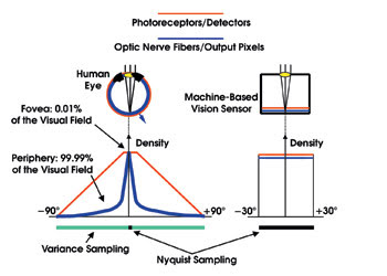
Figure 1. One difference between the human eye and machine-based image sensors is that, in the eye, the photoreceptors are distributed nonuniformly over the visual field. In a machine-based image sensor, the entire field of view is covered by a uniform array of detectors.
In a machine-based image sensor, the entire field of view is covered by a uniform array of detectors, each having, in effect, a unique output path (Figure 1). In the eye, on the other hand, the photoreceptors are distributed nonuniformly over the visual field, and it is only over the extremely small foveal area that each photoreceptor has its own unique output path, which is an optic nerve fiber. Away from the fovea, the sampling frequency (defined by the optic nerve fiber density) is much lower than the highest spatial frequency (defined by the photoreceptor density). This is the characteristic feature of variance sampling. Therefore, almost all of the sampling performed by human vision can be modeled by variance sampling, but not by Nyquist sampling.
Machine vision systems based upon Nyquist sampling seek to emulate the vastly superior recognition capability of human vision, yet derive a completely different type and quantity of visual information. In many cases, it may be possible to perform automatic recognition much more effectively and efficiently using low-pixel-density variance sampling.
Machine vision
Machine vision uses two basic recognition techniques: geometric vector matching, where edges within the object are identified, and normalized gray-scale correlation, where the information used is the intensity, or gray level, of all of the pixels in the image. Variance sampling, which is pixel-based, is applicable to normalized gray-scale correlation but not to geometric vector matching.
With normalized gray-scale correlation, object recognition is effected by cross-correlating a sensed gray-scale image of the object (generated by Nyquist sampling) with a reference image that defines the object. Dividing by the intensities of the two images normalizes the cross-correlation result, indicative of how similar they are. The object can then be recognized independent of its overall illumination level. But nonlinear changes in illumination are not corrected by this global normalization.
A fundamental problem with this technique is that, for a variety of practical reasons (such as slight differences in pose, parallax effects), the sensed image of the object to be recognized is never exactly the same in point-by-point detail as the reference image that defines that object. To capture the high-resolution information essential for recognition, Nyquist sampling, with its high-sampling density, generates a mass of point-by-point detail. Point-by-point detail that does not correspond is irrelevant and obstructive because it does not represent what is known of the object and, therefore, cannot contribute to its recognition.
What is needed for object recognition with normalized gray-scale correlation is a high-resolution representation of the object, limited in content to what is known of it. This representation is uniquely provided by a low-pixel-density variance image generated by variance sampling. A high true-match correlation coefficient is achieved because the object and reference variance images correspond despite their low pixel density, containing high-resolution information that enables one object to be discriminated from another.
It often will be necessary to register the object and reference images before performing normalized gray-scale correlation. This can be done readily with variance images because only approximate registration of the low pixel density is needed.
Once an object has been recognized, it may be necessary to precisely align it in some applications. This can be done by exact registration of object and reference variance images at progressively higher pixel densities (lower sampling factor) until high-pixel-density Nyquist images are used (SF – 1). High-resolution information is used at all steps in this variance-based pyramid processing action, assuring convergence to precise alignment.
Variance sampling
Variance sampling is implemented by simple preprocessing of a conventional digital image generated at any time by any conventional image sensor. Each variance pixel sample V(I,J) is computed as the variance of a subarray of SF × SF pixels in the input image CONV(X,Y) (Figure 2). A normalized variance image NV(I,J) also can be derived by dividing the variance sample V(I,J) by the mean sample M(I,J). The normalized variance image is dimensionless and thus has the important benefit of being nominally independent of scene illumination and, in particular, of nonlinear changes in brightness over the object.
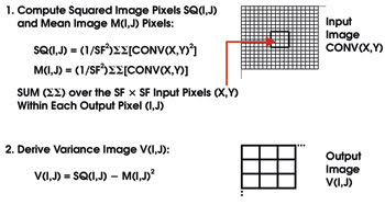
Figure 2. Each variance pixel sample [V(I,J)] is computed as the variance of a subarray of SF × SF pixels in the input image CONV(X,Y), where SF (sampling factor) is an important parameter of variance sampling.
In principle, low-pixel-density variance sampling could be performed directly in a special image sensor using a spatial modulation technique. Spatial modulation has been implemented in an IR sensor to perform a different, although related, low-pixel-density sampling. The benefit of spatial modulation in the IR case is that high-resolution sensing can be performed using an affordable and available low-density IR focal plane array.
However, in the visible spectrum, high-resolution CCDs are readily available and affordable, so there is no need to implement variance sampling in a special sensor. Instead, variance sampling can be performed for any desired SF value on the output from any standard image sensor by the processing action illustrated in Figure 2. The sampling operations involved are simple, and the processing load incurred is small compared with what would otherwise be required for recognition processing of high-pixel-density Nyquist images.
The basic problem with automatic object recognition by normalized gray-scale correlation is that the sensed image of the object is generally not exactly the same as the reference image that defines it. If they were, recognition by this technique would be easy. As with a jigsaw puzzle piece, the sensed image would either match a reference exactly or not match it at all.
However, if the sensed- and true-reference images are only slightly different, the true- and false-match cross-correlation coefficients may all be similar, and the true match then cannot be reliably identified. Low-pixel-density variance sampling overcomes this problem. Slight differences in point-by-point detail between the sensed and true reference images are suppressed by the low-pixel-density. Yet the high-resolution information that is essential for recognition is captured as variance within each pixel.
An experiment
A simple experiment can illustrate the superior recognition capability of low-pixel-density variance images when the sensed- and true-reference images are not exactly the same. The experiment starts with conventional (512 × 512) reference images of a car and a tank. The “unknown” object is the same tank image rotated by 10° (Figure 3). That rotation is a simple, but substantial, representation of the typical differences between the image of an unknown object and the reference image. The unknown image is normalized gray scale correlated with each of the two reference images (the car and the nonrotated tank).

Figure 3. An experiment using images of a car, a tank and a tank in a different orientation demonstrates the superior recognition capability of low-pixel-density variance images over conventional images.
The objective of this experiment is not to recognize the unknown image, but to compare the recognition capability of conventional and variance images. The metric (W) used to quantify recognition capability for both types of images is the difference between the cross-correlation coefficient (COR_TRUE) of the sensed image against the tank reference, and the cross-correlation coefficient (COR_FALSE) against the car reference: W = COR_TRUE – COR_FALSE.
In the ideal environment for this experiment, correct classification is indicated if W is simply positive, irrespective of its magnitude. However, in a real-world environment, a variety of artifacts and multiple references will combine to effectively introduce a background noise (w) into the recognition metric. In this case, the probability of correct classification is a function of (W-w)/w, and therefore it depends upon the magnitude of W; that is, the magnitude of W is a measure of recognition capability.
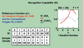
Figure 4. The results of an experiment comparing the recognition capability of variance images with that of conventional images as a function of pixel density show that the recognition metric (W) for low-pixel-density variance images (16 × 16 at n = 5) is almost two times greater than that of conventional images at any pixel density (n).
The value of W was computed in the experiment using variance and conventional images. This was done over a set of iterations (n = 1,2, . . 7) with pixel densities from 256 × 256 to 4 × 4 (Figure 4). It can be seen that the recognition metric W for low-pixel-density variance images (16 × 16 at n = 5) is almost two times greater than that of conventional images at any pixel density. The corresponding improvement in probability of correct classification in a real-world environment would be substantially greater because it’s a function of (W_VAR-w)/(W_CONV-w), rather than of (W_VAR/W_CONV).
This experimental result clearly demonstrates the superior recognition capability of variance images relative to that of conventional images when the sensed- and true-reference images do not correspond. Because the experimental result is not object recognition but a comparison of recognition capability between two image sampling protocols, variance and Nyquist, it is independent of artifacts of the particular patterns used (tank with background and car with no background), because any such artifacts apply equally to both sampling protocols.
Benefits
The primary benefit of low-pixel-density variance sampling for recognition is reliable recognition, even when the sensed image of the object and the reference image that define it differ because of pose differences, parallax effects, damage, design differences or differences within a class (when a single reference image defines a class of objects). In addition, normalized variance sampling offers immunity to nonlinear illumination (local variations in illumination over the object).
Variance sampling also provides a reduced processing load, because of the low pixel density, and a faster response time. An added benefit is that each reference image can cover a wider range of poses because of its low pixel density. Much less memory is needed to store each reference image, thereby enabling many more objects over many more poses to be represented in the reference memory.
These performance and implementation features may substantially improve the cost-performance ratio of object recognition, orientation sensing and defect detection in machine vision. Variance sampling can be used to enable a robot to learn its visual environment and then move and operate within it. It may be applied in medical imaging to allow recognition of human features whose patterns are not precisely definable. And it also may be applied for automatic facial and target recognition in security and military systems.
Meet the author
John Merchant is president of RPU Technology in Needham, Mass., and was formerly at Loral Infrared and Imaging Systems. He has a patent pending for the generation and application of variance images; e-mail: [email protected].