There is more to single-photon detectors than resolving single photons. Getting the most out of these devices requires a deeper understanding of quantum mechanics and detector design.
SLAWOMIR S. PIATEK AND EARL HERGERT, HAMAMATSU CORP.
Light transmits information about its emitter (source) and the medium of propagation.
If this information is relevant, the light can be detected for analysis — and it has been detected with increasing levels of sensitivity and resolution over the years. Today’s detectors have the ability to achieve single-photon resolution. Putting such capabilities into practical application is still not a trivial task, however, and can benefit from a deeper understanding of the principles of detection and single-photon resolution.
Over time, engineers have designed a multitude of photonic detection systems. For example, a spectroscopic system determines intensity as a function of wavelength, while an imaging system acquires a two-dimensional projection of a three-dimensional scene. The operation
of these and other detection systems broadly falls into four modes: analog, photon counting, coincidence, and integration.
In an analog system, the output from the sensor coupled to the front-end electronics manifests as a voltage or current as a function of time. This technique is typically employed when the incident light level is high enough so that the electrical pulses deriving from individual photons have a significant temporal overlap and, thus, cannot be distinguished individually.
In contrast, when individual electrical pulses are discernible, a user may instead opt for digital photon counting, a detection mode in which electrical pulses that satisfy certain threshold criteria are counted within a specified time interval.
Coincidence detection engages at least two detectors that are operating in sync. Detection of a photon is valid only when both detectors generate outputs within a certain time gate.
The integration mode of detection is conceptually similar to photon counting: The output is proportional to the number of photons absorbed within the assigned integration time. This mode is very common in imaging applications.
All of the above techniques are fraught with trade-offs, limitations, and subtle considerations, and they demand some expertise in optical, mechanical, and electronic design, as well as a clearer grasp of single-photon and photon-resolving detection methodologies.
The basics
Let’s assume the incident light impinging on a detector consists of square pulses, each of duration Tp containing, on average, N photons arriving with the repetition period Tr, such that Tr > Tp. If a detection system can discern the number of photons in each pulse, then it can be said to have a photon-number-resolving ability. Although this ability depends on the characteristics of both the front-end electronics and the sensor, it is the latter that is decisive.
If the sensor lacks the ability to resolve single photons, then not even ideal (noiseless) front-end electronics will qualify the system as capable of resolving photon numbers. It is tempting to state that a
sensor capable of detecting a single photon is also capable of resolving the number of photons, but such a statement would be false. Single-photon detection does not necessarily imply single-photon resolution, for two reasons.
First, the detector may have a binary response defined either as “one photon”
or a “no photon.” If two photons simultaneously strike the sensor, however, the
response will still register as “one photon.” A single-photon avalanche photodiode is an example of a detector belonging to this class.
Second, intrinsic noise in the detector — most notably, the noise due to the gain variation — can affect the output enough to create uncertainty as to the number of impinging photons. To illustrate this point, suppose that a single photon causes an amplitude of the output pulse to be A. For a noiseless detector, two concurrent photons yield an amplitude of 2A. However, if the gain of the sensor varies, say by a factor of two, then even individual photons can produce amplitudes ranging from A to 2A (Figure 1a).
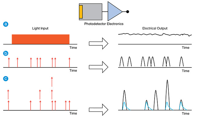
Figure 1. Three different input light conditions (left) and the corresponding detector outputs (right). Analog detection, in which the output is
a continuous function of, for example, voltage as a function of time (a). Photon counting, where the input consists of individually arriving
photons and the output of the corresponding electrical pulses (b). The responses of binary (blue) and proportional (black) detectors in response to multiphoton input delta pulses (c).
Courtesy of Hamamatsu.
The output of a photovoltaic sensor is defined by a voltage as a function of time produced by the photodetector and detection electronics. The voltage is proportional to the input radiant power and spectral sensitivity of the sensor. Figure 1b illustrates a photon-counting mode: The individual photons at the input give rise to the corresponding electrical pulses at the output. It is important to note that analog detection could still be utilized in this situation, though with some disadvantages.
Figure 1c explains the difference between a proportional and a binary sensor. The input is a sequence of delta pulses containing one, two, or three photons. A proportional detector outputs pulses (shown in black) whose amplitude is proportional to the number of photons. In contrast, a binary detector outputs pulses (shown in blue) of the same amplitude, regardless of the number of photons.
Photon counting offers several advantages over analog detection. Because the technique discriminates between the electrical pulses based on their amplitudes — in that an amplitude must be larger than a certain lower threshold and smaller than a certain upper threshold — the net count is less sensitive to noise. Common types of noise register as gain variation, electronic 1/f noise, output drift caused by changing
temperature, dark current, or sporadic events, such as cosmic ray hits.
The chosen integration time is central to the successful implementation of photon counting because its value affects the signal-to-noise ratio during detection, as well as the ability to detect variations in input power. A long integration time averages out changes in the incident radiant power. Assuming input power is constant, then the longer the integration time the larger the signal-to-noise ratio. For modulated input, the chosen integration time must satisfy Nyquist’s sampling theorem for the largest frequency component expected to be identified.
Another detection approach — that does not utilize integration techniques — is to timestamp detected photons and then plot a time-series histogram of the number of photons per time bin, the width of which will determine the largest frequency component in the modulation.
A proportional single-photon detector does not necessarily have the ability to resolve single photons. Figure 2 illustrates this important point. In it, a pulsed laser illuminates a proportional single-photon detector with δ pulses, averaging four photons each. The actual number of photons in a pulse follows the Poisson statistics, in which the probability P of seeing k photons in a pulse, with an average of λ, is given by the equation in the figure.
Assuming the detection electronics can measure an amplitude for each pulse, the amplitudes can then be plotted in a histogram.
The histogram in Figure 2a is for a
proportional detector that has a single-photon-resolution ability, whereas the Figure 2b histogram is for a detector that does not have this ability. Clearly demarcated columns can be seen in the Figure 2a histogram. And, if the quantum efficiency of the detector is 1, then, with enough trials, the histogram will resemble the Poisson distribution. Due to detector
and electronic noise, the columns in the Figure 2b histogram overlap, giving the net distribution shown in green. The comb-like appearance of this histogram is lost and so is the photon number resolution.
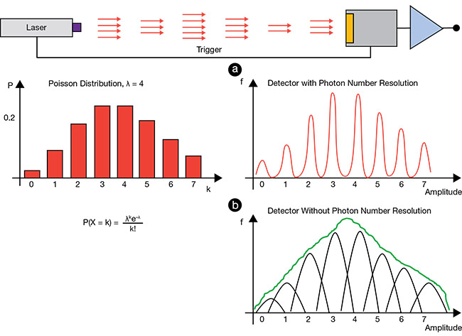
Figure 2. Photon number resolution. The detector receives pulses from the laser, with the mean number of photons per pulse λ. Due to Poisson statistics, the actual number of photons in the pulses varies. The Poisson probability distribution for λ = 4 (a, left), where k is the number of photons. A histogram of detections for a system that has a photon-number-resolving ability (a, right). A histogram that does not have the ability (b). The observed histogram (green). Courtesy of Hamamatsu.
The main attribute of a single-photon sensor is the presence of a positive feedback mechanism by which a single-
photon event leads to µ > 1 detection electrons, where the quantity µ is known as the gain. In addition to noise contributed by the detector’s front-end electronics, the stability of gain from event to event is the key factor for resolving the number of photons. As the average number of photons per pulse increases, the photon-resolving ability will eventually be lost, most often due to detector nonlinearity and saturation or, equivalently, a limited dynamic range.
These details describing photon-resolving capabilities — as well as the value of the capability — are illustrated by the three subsequent application examples.
The Hong-Ou-Mandel experiment
A two-photon interference experiment1, illustrated in Figure 3, helps demonstrate the benefits of a photon-number-resolving detector. The experiment is a variation on the seminal Hong-Ou-Mandel two-photon interference experiment2.
In the experiment, light from a continuous-wave laser pump, with frequency ω, is incident on a nonlinear optical crystal for collinear downconversion that, owing to the spontaneous parametric downconversion, produces orthogonally polarized photon pairs. Because the photons in the pair result from an energy- and momentum-conserving process and were created simultaneously, they are entangled. They are called signal (frequency ω1) and idler (frequency ω2) such that ω = ω1 + ω2 and ω1 ≥ ω2. For a degenerate downconversion, the case would be ω1 = ω2.
After wavelength and spatial filtering, the pairs are incident on a compensator, which allows control over the relative time delay between the two photons in the pair. The photons are eventually incident on a nonpolarizing 50/50 beamsplitter that, at its outputs, has two Glan-Thompson polarization analyzers aligned in such a way as to make the two photons indistinguishable in polarization. The time delay produced by the compensator controls the degree of indistinguishability between the photons. By varying the time delay, it becomes possible to achieve a situation in which the photons are maximally indistinguishable and will always exit the beamsplitter as a pair from either one of the two output ports.
Two transition-edge sensors, one for each output port, are used to detect the pairs. The detector operates at a cryogenic temperature close to absolute zero in a transition region where its resistance steeply decreases as the temperature
approaches 0 K. The detector is bolometric and capable of photon number resolution.
According to quantum mechanics, two photons that have the same wavelength, polarization, spatial extent, and temporal extent are said to be indistinguishable. If two such photons are incident on the two input ports (one photon per port) of a 50/50 nonpolarizing beamsplitter, they always emerge together, though randomly, at one of the two output ports.
This behavior was indirectly confirmed in the famous Hong-Ou-Mandel experiment. The confirmation was indirect because the photodetectors that the experimenters used did not have a photon-number-resolution ability. So, the emerging photon pairs could not have been directly detected. The photodetectors in the experiment depicted in Figure 3, however, do have this ability, which would allow direct detection of the emerging pairs.
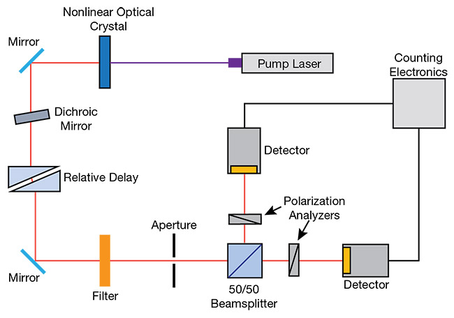
Figure 3. An experimental setup of the two-photon interference experiment to observe photon pairs exiting one of the two output ports of the beamsplitter. Adapted with permission from Reference 1. Courtesy of Hamamatsu.
Quantum OCT
Quantum optical coherence tomography (OCT) further helps to illustrate the
principles and benefits of photon counting. The schematic in Figure 4 demonstrates coincidence detection of entangled photons to probe the structure of a specimen. The schematic shows a nonlinear optical crystal pumped with a laser to produce entangled photon pairs. The signal photon takes path 1 while the idler photon takes path 2.
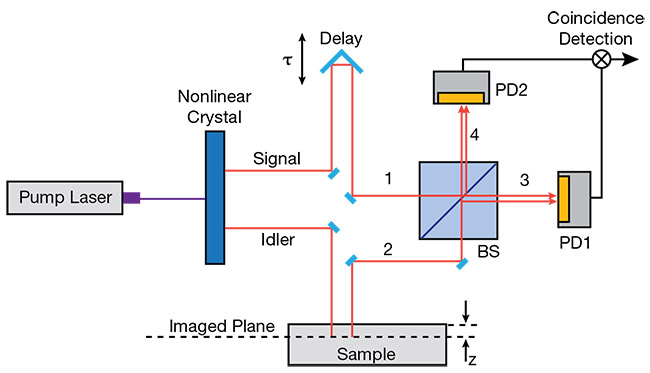
Figure 4. The experimental setup for quantum optical coherence tomography. Adapted with permission from Reference 3. Courtesy of Hamamatsu.
Path 1 leads the photon to an optical delay and to the first input of the beamsplitter; path 2 leads the other photon to the sample and to the second input of the beamsplitter. If the path lengths differ substantially, the photons are distinguishable, which means that the signal photon can exit ports 3 or 4 with the same probability, and the idler photon can also exit ports 3 or 4 with the same probability, leading to a high rate of coincidence detection.
However, if the delay is adjusted so that path 1 has the same optical length as path 2, the signal and idler have a high degree of indistinguishability and will exit the beamsplitter as a pair, either at port 3 or 4.
Consequently, the rate of coincidence drops to the minimum because destructive interference between the signal and idler suppresses the outcome, where one photon exits port 3 and the other port 4. The quantum version of OCT, compared to its classical counterpart, offers higher sensitivity to weakly reflecting structures and higher lateral and longitudinal resolutions.
Fluorescence microscopy
The final application example, entangled-photon fluorescence microscopy, illustrates the use of a single-photon detector operating in a photon-counting mode.
The setup in Figure 5 shows a quantum version of the classical two-photon fluorescent microscope. Here, the laser-pumped nonlinear optical crystal produces two divergent (signal and idler) beams of entangled photon pairs. Using mirrors, the beams are crossed in the specimen, resulting in the formation of the entanglement volume, in which a fluorescent molecule can be excited by absorbing two entangled photons. The subsequently emitted fluorescent photon is detected by a single-photon detector operating in a photon-counting mode. The mirrors control the location of the entanglement volume, enabling a 3D scan of the specimen. Because the rate of two-photon absorption is higher for entangled photons, compared to uncorrelated photons, lower photon densities are needed to excite fluorescence, resulting in lower bleaching and higher lateral and longitudinal resolution.
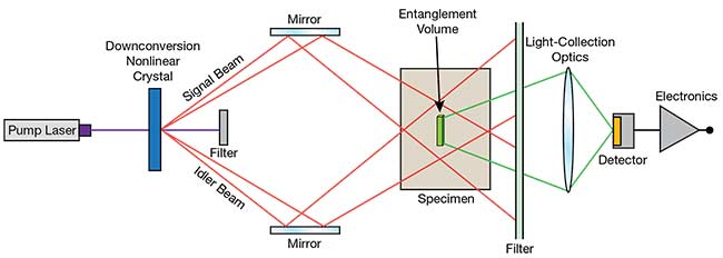
Figure 5. The experimental setup of a quantum two-photon fluorescent scanning microscope. Adapted with permission from Reference 4. Courtesy of Hamamatsu.
The prominence of single-photon detectors will only increase as quantum applications such as the ones described become more mainstream.
Meet the authors
Slawomir S. Piatek, Ph.D. is senior university lecturer of physics at New Jersey Institute of Technology and a science consultant for Hamamatsu Corp. He earned a doctorate in physics from Rutgers, The State University of New Jersey; email: [email protected].
Earl Hergert is a vice president of marketing at Hamamatsu Corp. in Bridgewater, N.J.
He has worked at Hamamatsu for 28 years; email: [email protected].
References
1. G. Di Giuseppe et al. (2003). Direct observation of photon pairs at a single output port of a beamsplitter interferometer. Phys Rev, Vol. A 68, No. 063817.
2. C.K. Hong et al. (1987). Measurements of subpicosecond time intervals between two photons by interference. Phys Rev Lett,
Vol. 59, No. 2044.
3. A. Abouraddy et al. (2002). Quantum-optical coherence tomography with dispersion cancelation. Phys Rev, Vol. A 65, No. 053817.
4. M.C. Teich and B.E. Saleh (1997).
Entangled-photon microscopy. Cesk cas Fyz, Vol. 47, No. 3.