By providing direct quantification of the positions of fluorophores, the method enables detailed in vivo investigation into molecular clustering, count and density.
CARL EBELING, BRUKER FLUORESCENCE MICROSCOPY
Fluorescence microscopy has proven itself to be an indispensable method in the modern biological toolkit. The use of visible-wavelength fluorophores allows for relatively noninvasive imaging. While the resolution of conventional optical microscopy cannot rival that of electron, atomic force or near-field scanning optical microscopy methods, the unrivaled specificity of the technique allows for the imaging of nearly any biological target.
With the advent of optical far-field superresolution technologies, researchers can combine the flexibility of optical microscopy with the image resolution required to ascertain biological structure and function at the nanoscale. One method, single-molecule localization microscopy, allows for the direct quantification of the positions of fluorophores under investigation and in the process opens up new avenues of statistical analysis to extract biologically relevant information. It is essentially the combination of two processes: optically controlling the fluorescent state and subsequent localizing on individual molecules.
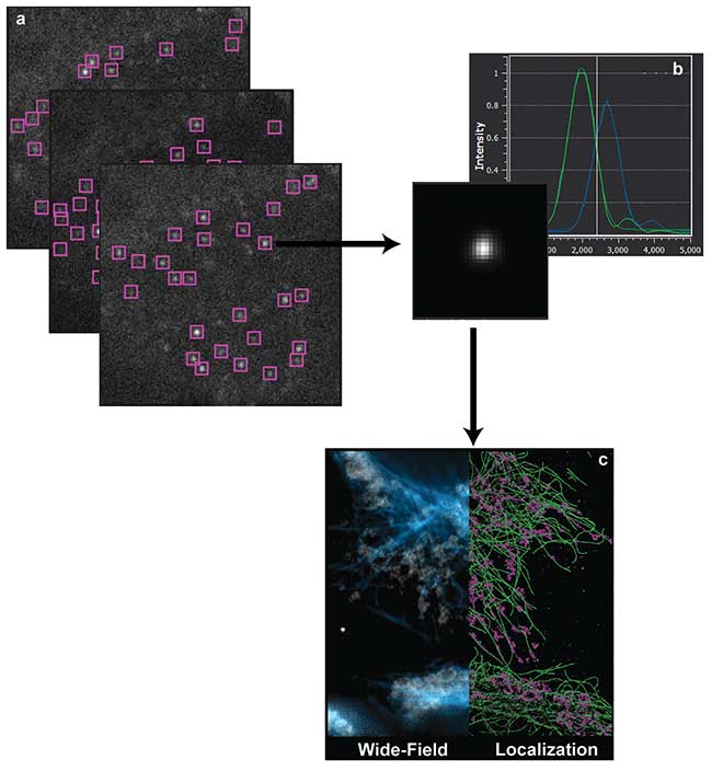
Figure 1. Single-molecule localization microscopy (a). Sequential imaging and recording of sparse stochastic subsets of individual molecules. This process accumulates data over thousands of frames with a sparse subset of active fluorophores spatially separated from its nearest active neighbor by more than the diffraction limit (b). Localization analysis occurs over every region of interest, and the XYZ positions of the molecule’s estimated position are tabulated (c). Visualization of the localization data set (right) compared to the reference diffraction-limited wide-field image (left). Courtesy of Dr. Manasa Gudheti and Dr. Carl Ebeling.
Ten years after its discovery, localization microscopy is in a maturation phase where it is becoming more of a routine analysis sequence in an experimental assay. Localization microscopy has become an important tool in the studies of synaptic function and structure; protein organization and arrangement in cellular vesicles and membranes; virus structure and organization; cytoskeletal networks; transcription factor distribution within the cell; and DNA organization and chromosomal structure.
Technological advances with camera sensitivity in the 1990s allowed for the foray into single-molecule imaging and characterization, where isolated single fluorescent molecules could be individually measured and analyzed. Since the characteristic photon distribution emitted from a point source onto a detector through an optical system is well known, analyzing the photon distribution, or the point-spread function (PSF), of single isolated fluorophores allows for the determination of the position of the emitter to a precision an order of magnitude lower than the approximately 200- to 300-nm-wide spatial extent of the photon distribution on the detector.
While the diffraction barrier is not optically surpassed per se, analyzing a single molecule allows for spatial information regarding the fluorophore’s location to be extracted from the photon signal at a level well below the spatial extent of the PSF itself. The uncertainty in the location of the fluorophore will scale as the inverse of the square root of the collected photons, which for bright fluorophores or point sources can yield a 100- to 1000-fold increase in the precision of the estimation of the fluorophore location. Thus, for single molecules isolated in vitro, the position of the fluorophore can be localized spatially to a few nanometers.
The natural progression from imaging single molecules in vitro is to image them in biological specimens. However, isolating densely packed individual fluorophores in vivo is much more complicated than spatially isolating them in vitro through controlled experimental protocols. Determining the spatial location of numerous densely packed fluorescent molecules is not possible because of the indistinguishability of photons. With numerous molecules fluorescing at once, it is impossible to determine which portion of the signal on the camera is coming from given individual molecules; only the ensemble average is recorded.
The conceptual analog of spatially isolating single molecules in vitro is to enlarge the dimensionality of the recording space in vivo to a degree larger than is required for conventional optical recording. Adding dimensionality to the recording space allows for the individual isolation of single molecules and the determination of the positions below that of the diffraction-limited optical volume in which they reside on the detector. This multiplexing can be achieved through either temporally or spectrally isolating single molecules apart from the ensemble1.
Controlling the optical state of specific fluorophores in vivo, either through low-level ultraviolet illumination or photo-chemical manipulation of the chromophore, is key to being able to isolate individual molecules from the sample ensemble2. Such optical control amounts to either stochastic temporal photoactivation or spectral photoswitching. By actively controlling the fluorescent state of individual molecules in the biological sample through strict photoactivation control, a small spatially isolated subset of the total number of fluorophores can be imaged and photobleached in the lifetime of a camera frame. Sequential imaging and recording of individual stochastically determined subsets allows for the spatial determination of each fluorophore present in the sample (Figure 1).
By extending the recording to thousands or hundreds of thousands of frames, the underlying biological structure is reconstructed. Thus, subdiffraction-limit-sized organelles, which would otherwise be indistinguishable if all of the fluorophores were on simultaneously as an ensemble, can be spatially resolved.
Single-molecule localization microscopy was pioneered using both photoactivatable and photoswitchable fluorescent proteins ((F)PALM)3,4 and organic dyes ((d)STORM)5. Because of the nature of the technique, localization microscopy does not generate a conventional image at the end of the recording and localization sequence. Rather, the processed data is a two- or three-dimensional array of molecular positions derived from the analysis of the thousands or millions of individual PSFs recorded. In this processing stage, candidate events can be discarded that do not meet certain convergence criteria for the localization algorithms, such as more than one fluorophore being active in a diffraction-limited volume.
Conventional and superresolution optical techniques rely on capturing the fluorescence signal through the optical system of the microscope, assigning it to camera pixels or to a detector, and then rendering an image. While methods such as stimulated emission depletion (STED) or 4Pi microscopy confine the fluorescence emission volume to a size lower than the conventional diffraction limit, the signal on the detector is still an aggregate of multiple fluorophores.
Conversely, localization microscopy must computationally render an image from the localization positions within the data set (Figure 2a). The generated images reveal a much higher degree of structural detail compared to conventional microscopy: Molecules are imaged individually and their coordinates are recorded to generate a superresolution image (Figure 2b). However, the most significant biological information arises from analysis of the spatial arrangement of the molecules and of the interaction of the molecular ensemble as a whole.
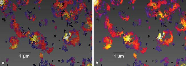
Figure 2. Image generation from single-molecule location data, sample of Cy3B-labeled mitochondrial protein TOM20 in BSC1 cells (a). Each localization is rendered as a single sphere of constant size. This type of image showcases what single-molecule localization microscopy inherently is, namely the mapping of the molecular positions of the biological target (b). Each molecular position is convolved with a Gaussian intensity distribution, yielding a more conventional image to the data set. Recording, localization, image generation and statistical analysis all performed on Vutara SRX software. Courtesy of Dr. Manasa Gudheti and Dr. Carl Ebeling.
Generating an image from localization data is not required to extract metrics of biological features. Analyzing the localization data directly can answer pertinent physiological questions related to protein clustering and aggregation; the distribution and interaction of target proteins or organelles; and colocalization of two separate cellular structures. The arrangement of the recorded molecular positions is quantifiable, enabling investigations into the degree of molecular clustering, cluster size, shape, molecular count and density. One of the most common biological questions concerns the level of clustering involved in the molecular distribution of the localization data, and how the data set forms aggregates that can be correlated into interacting units. (See sidebar for application notes.)
Systematically being able to identify clusters based upon molecular densities and spacing allows for reproducible analysis of data across numerous experiments and assays, such as drug treatments and their effects on protein, DNA and RNA distribution within cells. Once the clusters have been identified, the particle counts, volume and shape can be calculated to yield representative biological information (Figure 3). For example, the direct imaging of genomic structure is possible through localization microscopy6. The conformational shape of the chromosome and its role in levels of gene expression can be studied, with small regions of the chromosome forming a unique clustering event. The morphology of the clusters, in turn, can help elucidate the effect of conformational shape of DNA to levels of gene expression in the cell.
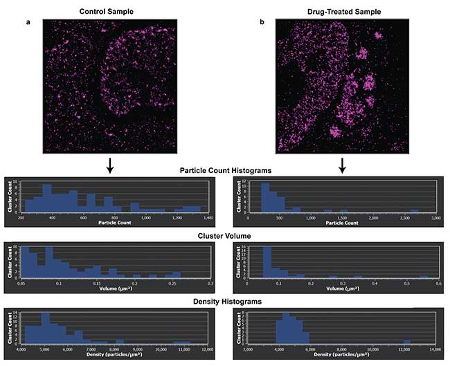
Figure 3. Density analysis of the clusters formed from two samples labeled with Alexa Fluor 647 HuR-RNA binding protein targeting stress granules. Control sample and cluster density (a). Density histogram of sample treated with DDT for one hour, inducing stress granules in the sample (b). Performing cluster analysis on the samples shows the effect of DDT on the cluster density. Samples imaged on Bruker Vutara 352 microscope. Recording, localization, image generation and statistical analysis all performed on Vutara SRX software. Courtesy of Alyson Hoffman & Chris Nicchitta, Duke University School of Medicine.
In addition, the surface distances between the groups of clusters can be calculated to establish the characteristic spacing between clusters or the colocalization and interaction distances between two biological targets. The clusters within the data set can be analyzed pair-wise, allowing for examination of the spatial relationships between all clusters. One study into possible causes of acute interstitial edema, for example, focused on the localization of potassium channels in the perinexus tissue, where clusters of two protein complexes associated with each feature were analyzed to determine the most frequent intercluster distances between the two proteins. These distance metrics were then used to develop hypotheses on the interaction between the two complexes with each other in the cellular environment7.
Because localization microscopy enables statistical calculations on molecular distributions, the advancement of data analysis goes hand in hand with localization microscopy imaging. Having a high-resolution image is critical to visualizing the spatial interaction of cellular phenomena at biologically relevant length scales, but having quantifiable metrics based upon the localization data to validate or disqualify experimental hypothesis is at least equally important.
Challenges do exist with localization microscopy data analysis. For one, each localization in the data set is a unique event with an associated uncertainty with the estimation of the spatial coordinates of the fluorophore. These uncertainties should be accounted for during analysis, such as the inclusion of localization uncertainty in pair correlation or colocalization formulas and in resolution analysis calculations. In addition, there is the question of sampling density or sampling number: Counting too few molecules may not adequately reconstruct the targeted biological structure or result in a partial statistical interpretation because of small sampling sizes. Issues such as fluorophore detection efficiency; target binding affinity and efficacy of the biological probe; and physiological alteration because of fluorophore labeling are all important experimental parameters that must be considered by researchers using localization microscopy.
For the academic researcher, commercial single-molecule localization platforms must be able to capture, localize and visualize localization data, and generate high-quality images. Equally as important, however, the platforms must be able to handle the computational analysis involved in the characterization of the data sets in an easy and straightforward manner. The investigative challenges and questions being asked in the biological sciences should not be limited by localization microscopy instrumentation’s lack of ability to analyze data in order to generate the statistical analysis required for evidence-based conclusions. To be considered a truly complete localization microscopy system, an instrument should be able to easily acquire data in the appropriate experimental conditions, localize the raw data, visualize the data streamline and generate reproducible, quantifiable statistical metrics.
Meet the author
Carl Ebeling is a worldwide applications scientist at Bruker Nano Surfaces in Salt Lake City. In 2010, while completing his Ph.D., he began to work for Vutara, a startup microscopy company based at the University of Utah that commercializes 3D localization microscopy. Bruker acquired Vutara in July 2014. Upon completing his thesis, Carl began to work full time for Bruker as an applications scientist, helping to support the establishment of the Vutara superresolution microscope in academic research and industry worldwide; email: [email protected]
References
1. E. Betzig (1995). Proposed method for molecular optical imaging. Opt Lett, Vol. 20, Issue 3, pp. 237–239.
2. R.M. Dickson et al. (1997) On/off blinking and switching behaviour of single molecules of green fluorescent protein. Nature, Vol. 388, pp. 355–358.
3. E. Betzig et al. (2006). Imaging intracellular fluorescent proteins at nanometer resolution. Science, Vol. 313, pp. 1642–1645.
4. S.T. Hess et al. (2006). Ultra-high resolution imaging by fluorescence photoactivation localization microscopy. Biophys J, Vol. 91 Issue 11, pp. 4258–4272.
5. M.J. Rust et al. (2006). Sub-diffraction-limit imaging by stochastic optical reconstruction microscopy (STORM). Nat Meth Vol. 3, pp. 793–795.
6. B.J. Beliveau et al. (2015). Single-molecule super-resolution imaging of chromosomes and in situ haplotype visualization using Oligopaint FISH probes. Nat Commun, Vol. 6, p. 7147.
7. R. Veeraraghavan et al. (2016). Potassium channels in the Cx43 gap junction perinexus modulate ephaptic coupling: An experimental and modeling study. Pflugers Arch, Vol. 468, Issue 10, pp. 1651–1661.
Working With Statistical Analysis
One direct application of statistical analysis on localization data is the use of Ripley’s K functions to determine the distribution and clustering characteristics of, as an example, cellular membrane proteins. Calculating the difference between the normalized Ripley’s L function and the value of the radial search, L(r) − r, will produce a characteristic peak in the curve at the radius of clustering of the proteins1 (Figure 1a). The functional behavior is such that the distribution will decay past the boundary of the cluster, allowing for statistical determination of the cluster size from the ensemble data.
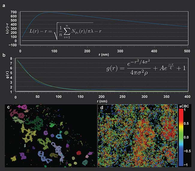
Figure 1. Ripley’s K analysis, L(r) − r, (shown on the plot), for a clustered data set (a). The peak value of the curve relates to the cluster boundary. For the Ripley’s K, n is the number of analyzed points, r is the radial offset, and λ is the number of localizations per volume. Pair correlation curve with experimental data shown in blue, with a best-fit in green (b). Function shown on plot for reference. The characteristic decay length, ξ, can be extrapolated from the best-fit decay curve. For the pair correlation function, r is the radial offset, σ is the standard deviation of the localization precision, and ρ is the average localization density. Visualization of a data set shown colored by cluster (c). Example of coordinate-based colocalization analysis, with the color scaling indicating degree of colocalization between two probes (d).
Another approach for determining cluster size is through the use of pair correlation functions. Pair correlation analysis offers the ability to quantify parameters such as spatial organization, clustering size and density in a data set without needing a determination of exact protein numbers (the case when imaging with organic dyes). Pair correlation functions allow for the incorporation of multiple blinking events of the same protein and the localization uncertainty, allowing for accurate modeling of the experimental conditions. Characteristic cluster sizes can be extracted from fitting pair correlation functions to characteristic decay curves (Figure 1b).
Cluster analysis allows for the localization data to be grouped into distinct units, representing underlying biological structures (Figure 1c); such grouping is a first level of analysis. Once the localizations are organized by cluster, cluster-related metrics, such as center-to-center or surface-to-surface distances2, can be calculated pair-wise over the clusters to give distributions of interaction distances between the biological features. This can be useful, for instance, in studying pharmacological effects on cellular organization or response, to see if drug treatments effect distances separating cellular sub-units.
Superresolution microscopy can provide deeper insights into protein colocalization compared to conventional microscopy, where colocalization can only be determined down to the diffraction limit, two orders of magnitude larger than the proteins themselves. With localization microscopy, coordinate-based colocalization algorithms can be applied to the data set, where the proximity of localization distributions of two probes are evaluated against each other and individually quantified as rank-order correlation values3 (Figure 1d). While this is similar to the standard Pearson coefficient, it is a more accurate representation of the colocalization of two biological targets due to the estimation precision of localization microscopy.
References
1. M.A. Kiskowski et al. (2009). On the use of Ripley’s K-function and its derivatives to analyze domain size. Biophys J, Vol. 97, Issue 4, pp. 1095–1103.
2. R. Veeraraghavan and R.G. Gourdie (2016). Stochastic optical reconstruction microscopy-based relative localization analysis (STORM-RLA) for quantitative nanoscale assessment of spatial protein organization. Mol Biol Cell, Vol. 27, Issue 22, pp. 3583–3590.
3. M. Georgieva et al. (2016). Nanometer resolved single-molecule colocalization of nuclear factors by two-color super resolution microscopy imaging. Methods, Vol. 105, pp. 44–55.