Gerald C. Holst, JCD Publishing
If we were to estimate the output of a CCD or thermal camera, we would typically draw an image over the detectors, aligning the image with the detector axes. We show it this way because it’s easy to draw; using quadrille graph paper, we simply follow the lines. In addition, symmetrical figures are easy to analyze. In the lab we can align a target with the detector array and easily verify our symmetrical drawings experimentally.
Not so in the real world. Take, for example, a web inspection facility where parts are randomly located on a moving conveyor belt. Here, the image can fall on any part of the detector, introducing phasing effects that are not obvious when we make our symmetrical drawings. It would be a lucky shot to achieve perfect alignment.
This variation in location leads us to wonder: What is the smallest image — flaw, blob or bar — that can be detected? And what is the minimum number of pixels required across the target?
Three-step process
It is important to understand how a camera system processes an image. First, the optics produce an image on the detector array. The detector output is proportional to the amount of light impinging on the active surface; i.e., detectors spatially integrate the signal, and each detector’s output is a single number. This means that the edge of an image cannot be precisely determined. We can only say that the edge falls somewhere on the detector. Second, the output of all the detectors is placed within a data array. Image-processing algorithms operate on this array. And finally, the array is converted into a visible image by a monitor or a printer.
Consider a circular flaw whose image just fills one detector. Suppose the output of each detector is digitized by an 8-bit analog-to-digital converter (256 gray levels). Because the area of a circle is πr
2, the maximum output of the array is:
| 0 |
0 |
0 |
0 |
| 0 |
200 |
0 |
0 |
| 0 |
0 |
0 |
0 |
| 0 |
0 |
0 |
0 |
If the image shifts by half a detector width both horizontally and vertically, the outputs are:
| 0 |
0 |
0 |
0 |
| 0 |
50 |
50 |
0 |
| 0 |
50 |
50 |
0 |
| 0 |
0 |
0 |
0 |
Is it possible for an image processing algorithm to detect this flaw? Typically a threshold would be selected to discriminate the target from its background. A high threshold avoids false positive identifications. If the threshold is set at 25, the flaw will appear as either one or four pixels; but if the threshold is set at 100, the flaw will appear as one pixel in the first case and will not be present in the second.
From this analysis, it is clear that spatial sampling introduces ambiguity of one detector width. A small blob may appear as one or two elements wide and one or two elements high. Depending on the phase, the flaw may be 1 × 1, 1 × 2, 2 × 1 or 2 × 2. It is important to note that after thresholding, the distorted (no longer circular) may be eliminated.
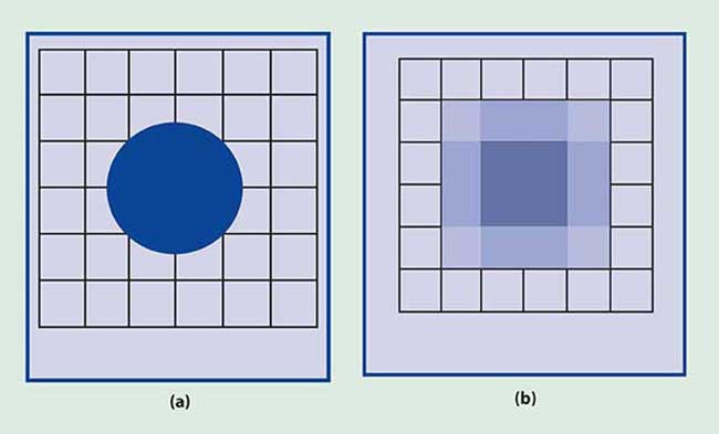
Figure 1. The intensity of a circular flaw with a diameter of three detector widths appears uniform (a) until it is reproduced by a printer or computer monitor (b), where edge location becomes ambiguous and the displayed image is no longer circular.
The image generally covers several detectors. In the instance of a circular flaw whose image diameter is three detector widths and the flaw is centered on the junction of four detectors (Figure 1a), the digitized detector outputs are:
| 0 |
0 |
0 |
0 |
0 |
0 |
| 0 |
2 |
97 |
97 |
2 |
0 |
| 0 |
97 |
255 |
255 |
97 |
0 |
| 0 |
97 |
255 |
255 |
97 |
0 |
| 0 |
2 |
97 |
97 |
2 |
0 |
| 0 |
0 |
0 |
0 |
0 |
0 |
When the flaw is reproduced by a computer monitor or printer (Figure 1b), the image is no longer circular and the edge location is ambiguous. Although the blob’s intensity is uniform, the displayed image has varied intensities.
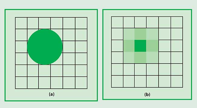
Figure 2. The edge location of a circular object (a) becomes ambiguous after detection (b). Image processing algorithms can estimate the flaw’s centroid.
If the same blob is centered on a detector (Figure 2a), the digitized detector outputs are:
| 0 |
0 |
0 |
0 |
0 |
0 |
| 0 |
135 |
248 |
135 |
0 |
0 |
| 0 |
248 |
255 |
248 |
0 |
0 |
| 0 |
135 |
248 |
135 |
0 |
0 |
| 0 |
0 |
0 |
0 |
0 |
0 |
| 0 |
0 |
0 |
0 |
0 |
0 |
The image of the flaw (Figure 2b) allows its center to be estimated, but its precise location remains unknown.
If a threshold greater than 248 is selected, the flaw can appear one or two pixels wide, and if a threshold less than 2 is used, the flaw width appears as three or four pixels. With these two thresholds, the blob appears as a square. Intermediate threshold values produce a cross.
As the shape of the object changes, the values in the data array also change. In the case of a bar-code reader, where we have conveniently centered the bars on the detectors (Figure 3), the data array is:
| 0 |
0 |
0 |
0 |
0 |
0 |
| 0 |
128 |
0 |
128 |
0 |
0 |
| 0 |
128 |
0 |
128 |
0 |
0 |
| 0 |
128 |
0 |
128 |
0 |
0 |
| 0 |
0 |
0 |
0 |
0 |
0 |
| 0 |
0 |
0 |
0 |
0 |
0 |
These bars can be easily discerned by all image processing algorithms, but bars are never aligned perfectly. With the same bars rotated 20° (Figure 4), the following data set results:
| 0 |
0 |
0 |
0 |
0 |
0 |
| 0 |
122 |
12 |
122 |
12 |
0 |
| 0 |
64 |
64 |
64 |
64 |
0 |
| 0 |
12 |
122 |
12 |
122 |
0 |
| 0 |
0 |
0 |
0 |
0 |
0 |
| 0 |
0 |
0 |
0 |
0 |
0 |
One big blob
Admittedly, Figures 3 and 4 illustrate a worst-case scenario. The bars appear at the array’s Nyquist frequency where they are nearly unrecognizable. In this case, the bar pitch (center-to-center spacing) is equal to twice the detector pitch. By moving aligned bars (Figure 3) horizontally by half a detector width, the data array will have four contiguous elements, each with a value of 64, and the bars will appear as one big blob. Phasing effects are most dramatic at the Nyquist frequency.
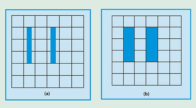
Figure 3. The vertical bars are separated by one detector width; the bar width is half a detector width (a). The output (b) remains constant for any location that fully encloses the bar.
The Nyquist frequency is often used as a measure of performance to indicate the smallest flaw spacing that can be detected. This is appropriate when the flaw is perfectly aligned to the detector axes. However, phasing effects force a more conservative approach. The smallest flaw spacing probably should be twice the Nyquist frequency; i.e., have a four-pixel spacing.
The minimum number of pixels on an image depends on the task. With machine vision systems, there must be a sufficient number of pixels for the computer algorithm to identify the target with some accuracy. The computed image size depends on both phasing effects and the threshold set in the algorithm. Robust image processing algorithms generally require flaws that are at least three pixels wide, with five-pixel flaws easy to analyze.
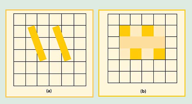
Figure 4. Two bars tilted at 20° (a) have a stair-step appearance in the displayed image (b).
A clear distinction must be made between system resolution and the ability to discern real objects. Resolution is a measure of the smallest blob that can be faithfully detected. As shown in the first example, a blob less than one detector width will always appear as one full pixel, assuming perfect alignment. Here the system is said to be detector-limited. The appearance of multiple bars (Figures 3 and 4) depends on resolution, phase and the relationship between the bar pitch and the detector pitch. Detecting nearly circular biological cells is quite different from reading bar codes.
TABLE 1.
| |
|
|
Average |
|
Typical Detector |
|
Maximum f Number |
| |
|
|
Wavelength |
|
Size (µm) |
|
for Graphical |
| |
|
|
(µm) |
|
|
|
Analysis |
| |
|
|
|
|
|
|
|
|
Visible |
|
0.5 |
|
5 (1/4-in. format) |
|
4.1 |
| |
Visible |
|
0.5 |
|
10 (1/2-in. format) |
|
8.2 |
| |
MWIR |
|
4.0 |
|
20 |
|
2.0 |
| |
LWIR |
|
10.0 |
|
30 |
|
1.2 |
A final note
Graphical analysis assumes that the optical blur diameter is small compared with the detector size (the definition of a detector-limited system). For diffraction-limited optics, the Airy disc diameter is:
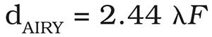
As the wavelength or the f number increases, the blur diameter increases. The maximum f number occurs when the Airy disc diameter is equal to the detector size. From Table 1, graphical analysis is generally valid for the visible region. As the optical blur increases, more pixels-on-target are required.
The relationship between detector size and optical blur diameter is discussed in "Camera Resolution: Combining Detector and Optics Performance".