Rüdiger Paschotta, RP Photonics Consulting GmbH
Developing active fiber devices based only on experimental tests is highly inefficient, often leading to time-consuming, expensive iterations in the laboratory. Working with a numerical model is the best way to learn how fiber devices work, how to optimize their designs and what their limitations may be.
Fiber amplifiers and lasers offer interesting advantages over more traditional laser types, including possible cost savings. However, the performance details often are more complicated than for bulk lasers as a result of strong saturation effects, consequences of a high laser gain and some peculiarities of quasi-three-level laser transitions. The design of such devices requires more than a few back-of-the-envelope calculations.
A trial-and-error approach easily can lead to time-consuming and costly iterations and nonideal results, not exploiting the full performance potentials. In most cases, the most efficient approach starts with numerical modeling, which allows the designer to analyze and solve problems and optimize the design quickly – before buying any expensive parts or spending substantial lab time. Diagnosing problems is much faster with a numerical model than in the laboratory because a model, unlike a real amplifier or laser, is fully “transparent.” It allows inspection of optical powers and excitation densities anywhere within the fiber and at any time, and the effects of considered design modifications can be simulated quickly.
Laser-active ion behavior
First, consider a single laser-active ion at some location in the fiber core being exposed to some number of optical fields (pump and signal waves, amplified spontaneous emission) with known intensities. Broadband amplified spontaneous emission (ASE) can be considered as a set of optical channels with various wavelengths. All these optical fields can drive transitions between electronic levels (more precisely, Stark level manifolds) of the ions, namely by absorption (from the ground state or from excited states) and by stimulated emission. Additional transitions can occur as a result of spontaneous emission and nonradiative effects such as multi-phonon emission and energy transfers between ions.
Figure 1 shows the simple example of an Er3+ ion, subject to a pump and signal wave, ignoring excited-state absorption and upconversion effects. Because the nonradiative transition from level 3 to 2 is very fast, it often may be considered as instantaneous, leading to a zero population density of level 3. The model may then include only the levels 1 (ground state) and 2 (upper laser level), and pumping is considered as transferring ions directly into level 2.
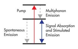
Figure 1. Simplified level scheme of Er3+ ions exposed to a pump and a signal wave. Images courtesy of RP Photonics Consulting GmbH.
The dynamics are governed by wavelength-dependent effective transition cross sections and the upper-state lifetime, apart from the optical intensities, and can be described with a set of rate equations. Powerful simulation software can even solve nonlinear rate equation systems for sophisticated systems; for example, with multiple metastable levels and energy transfers between various types of ions.
Some fiber manufacturers supply comprehensive spectroscopic data for their fibers, and as the industry matures, this will become the standard. Customers often hesitate to work only with guesses or trial and error, or to set up their own spectroscopic measurements. Ideally, directly usable data sets for various commercial fibers are provided together with simulation software, or they can be produced on demand within the user support.
Local gain or loss
Once the level populations have been calculated from the local optical intensities, the local gain or loss coefficient for the optical waves can be calculated. This also depends on the doping concentration profile of the fiber and the optical intensity profiles, which may be wavelength-dependent. The software should be able to calculate these intensity profiles with a mode solver or to work with profiles given by the fiber manufacturer. The fiber also may have some background loss, although this is negligible in many cases.
As an example, consider a signal and pump wave in a double-clad fiber. Figure 2 shows that the signal wave has a strong overlap with the single-mode fiber core, whereas the pump wave fills the whole undoped inner cladding, having only a small overlap with the doped core. The inner cladding actually supports a large number of modes, having substantially different overlap.
Precise modeling requires one to consider all modes separately, but in many cases it is sufficient to consider the whole pump wave as a single optical channel with a top-hat intensity profile – at least when strong mode mixing can be assumed; for example, resulting from a D shape of the inner cladding or from tight bending. As a result of the low core overlap in a double-clad fiber, the coupling of the pump wave to the ions often is much weaker than that of the signal wave, even if the pump cross sections are larger than the signal cross sections. This aspect has important implications for the performance details.
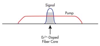
Figure 2. Transverse profiles of the intensities of signal and pump in a double-clad fiber.
Dynamic simulations
In some cases, the dynamic behavior of the system is of interest. In principle, this is relatively straightforward to simulate. Consider a simple case, where a signal pulse is amplified in a single pass through a fiber. Here, it often is not relevant for the model that various parts of the fiber “see” the signal pulse at different times. Propagation times can then be ignored. It is sufficient to numerically divide the pulse into small temporal slices and the fiber into small pieces, and then to propagate each temporal slice through all fiber pieces. When one slice travels through one fiber piece, it is amplified to some extent, and at the same time it extracts some of the stored energy; i.e., it changes the level populations. Later slices may thus obtain a reduced power gain, which can lead to pulse distortions.
In other cases, the propagation times cannot be ignored; e.g., they are essential for pulse formation in a Q-switched fiber laser. Here, one can use a numerical technique where each time step corresponds to the time required by light to propagate further by the length of one fiber piece. In each time step, the total field distribution in the laser resonator is moved forward by one fiber piece. Time delays outside the doped fiber also must be taken into account. Technically, this is more demanding, and such simulations often require more computation time because the method enforces the use of rather short time steps.
Figure 3 shows the result of an example simulation for an actively Q-switched fiber laser. Instead of a smooth pulse envelope, as is common for a bulk laser, the fiber laser emits a series of spikes because the lasing begins with amplified spontaneous emission, which is very unevenly distributed in the resonator because of the high gain. For the simulation, Q switching with a very fast modulator was assumed, but it would be easy to study the effects of slower switching, both on the temporal shape and on the power efficiency. Such simulations often create surprising results because it is difficult to anticipate all relevant details and effects before the simulation.
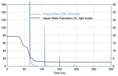
Figure 3. Temporal evolution of output power and averaged ionic excitation in a Q-switched fiber laser, simulated with the software RP Fiber Power. The separation of the spikes corresponds to one resonator round trip.
Steady state
Efficient calculation of the steady state for an amplifier or laser with constant input powers can be substantially more demanding than a dynamic simulation because the distributions of optical powers and ionic excitation densities influence each other. Therefore, a self-consistent solution is required.
First, we consider the simple case of an amplifier with a co-propagating pump and signal light and with negligible ASE. We already know all optical intensities at the input end, so we can calculate the excitations at this point. From that, we can calculate the local gain, which allows us to propagate the pump and signal power through a first short fiber piece. Step by step, we can propagate the powers and excitations all the way to the other fiber end. High precision is obtained simply by using small enough fiber pieces, and the computation time for a single-pass propagation can be very short, even when using 1000 pieces.
A more complicated case is that of an amplifier with a counterpropagating pump and signal. Here, we know only the local pump intensity at the pump input end, and only the local signal intensity at the opposite end. At no position do we initially know all optical powers. However, there is a relatively simple method to solve this problem, called the shooting method.
We begin at the signal input end; for example, with an initial guess for the residual pump power at this point. Then we propagate signal and pump through the fiber, using the fact that pump power rises in a backward direction according to the calculated level of pump absorption. At the pump input end, we will generally not obtain the true input pump power, but we can compare the propagated and the true pump input power and correct our guess accordingly. An appropriate one-dimensional root-finding mechanism allows us to find an accurate solution within a few iterations. Figure 4 shows the power distributions in an example case. The method also can be adapted to a linear fiber laser, where the backward-propagating signal wave is initially not known. Of course, the forward and backward signals must be made consistent with the end reflectivities.
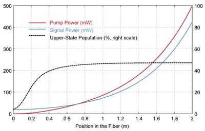
Figure 4. Distribution of steady-state pump and signal powers and the upper-state population in a fiber amplifier with a signal coming from the left side and a counterpropagating pump wave.
Although the shooting method is simple and efficient in the aforementioned cases, it is not practical in other cases, where we have multiple or even many backward-propagating fields. Here, we essentially would have to do a multidimensional root finding, which is substantially more difficult – particularly for high-gain cases, where we can have exponential dependencies. Because such cases often occur, it is desirable to have a method that can cope with them.
The basic principle can be that of a relaxation method. The simplest approach is to perform a sequence of steps, where one always first calculates the optical powers resulting from the currently assumed ionic excitations and then updates the excitations according to the local optical intensities. The problem is that the convergence properties depend strongly on the situation.
Although one may fine-tune an algorithm to be efficient in a specific situation, it is challenging to obtain reliable and efficient convergence in all situations, including high- and low-gain amplifiers (or amplifiers with different gain for different signals), ASE sources and lasers. However, it is possible to achieve this goal with a very refined algorithm. Elements of that can be to introduce some numerical “damping” to the calculated optical powers and to automatically adjust various numerical parameters according to the “observed” convergence properties. RP Photonics’ RP Fiber Power software makes that approach applicable to a vast range of situations. The user does not have to deal with the iterative procedure but can just enjoy the fast convergence
Learning by playing
The results of fiber amplifier and laser simulations often exhibit surprising features. In one example, shown in Figure 5, a single pump wave at 920 nm (and no signal) was injected into an ytterbium-doped fiber with no end reflections. Here, the distributions of pump power and upper-state population have quite surprising shapes because of ASE. Backward ASE becomes quite strong on the left side, extracting more than 40 percent of the pump power. It substantially pulls down the upper-state population, leading to increased pump absorption. The pump absorption is weaker at positions a little farther to the right, where ASE is weak. Roughly in the middle of the fiber, forward ASE becomes substantial, but then drops again as it is reabsorbed (because of the quasi-three-level nature of Yb3+). Additional diagrams, not shown here, would reveal that the spectral shape of ASE at various positions and traveling in different directions can be extremely different.
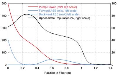
Figure 5. Distribution of pump and amplified spontaneous emission (ASE) powers and the upper-state population in an ytterbium-doped fiber pumped at 920 nm. RP Fiber Power software iteratively calculated a self-consistent solution of optical powers and ionic excitations. Less refined numerical algorithms could be plagued by convergence problems or require extensive computation time in such cases.
The behavior of the system can change profoundly when changing the fiber length or the pump wavelength. It would be very hard to fully understand and reliably predict the behavior of such a system without numerically simulating it. Even extensive measurements in the lab would not reveal the important role of forward ASE, as that has substantial power at positions only within the fiber, which are hardly accessible. Further, the behavior can be substantially more complicated when additional signal channels and/or end reflections are added.
Only numerical modeling can lead to quantitative understanding of device performance and, thus, is key to reaching high performance with the least possible development effort.
Meet the author
Dr. Rüdiger Paschotta is founder and president of RP Photonics Consulting GmbH in Bad Dürrheim, Germany; email: [email protected].