Replacing photomultiplier tubes with silicon photomultipliers can provide consistent and rapid quantitative imaging at the cellular level with limited loss of fluorescence intensity and high signal-to-noise ratio.
George Glekas and Joanna Hawryluk, Evident Scientific
When used appropriately, a laser scanning confocal fluorescence microscope is a valuable tool for researchers to make quantitative measurements in cells and tissue across various life sciences applications. The laser scanning confocal microscope’s ability to block out-of-focus light and thereby perform optical sectioning through a specimen allows the researchers to quantify fluorescence with very high spatial precision. However, generating meaningful data using confocal microscopy requires careful planning and a thorough understanding of not only this imaging technique but also the hardware capabilities of the imaging system itself.
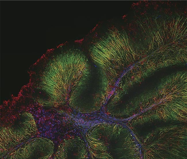
A mouse cerebellum captured on the FLUOVIEW FV4000 laser scanning confocal microscope featuring SilVIR detector technology, with neurofilament-heavy chain (green), myelin basic protein (red), and glutathione S-transferase pi 1 (blue). Fluorescence data is courtesy of Katherine Given at the University of Colorado. Image courtesy of Evident Scientific.
In confocal cell imaging applications, samples are labeled with fluorescent dyes and exposed to excitation light, in this case visible diode lasers, to obtain fluorescence signals. Excitation light, typically within the visible spectrum, can damage cells and lead to photobleaching of the expressed fluorescent dyes. Therefore, it is ideal to minimize sample exposure to excitation light. However, a decrease in the excitation light results in a decrease in the fluorescence signal. Autofluorescence, which is emitted from endogenous fluorescent molecules in living tissue, can further decrease the signal. These challenges make precise quantification of the fluorescent signal difficult.
Why intensity matters
Measuring the number of photons is the most accurate way to quantify very weak fluorescence light.
Although there are various definitions of the physical measurement of detected light, measuring the number of photons is the most accurate way to quantify very weak fluorescence light. Therefore, the simplest way to measure light intensity is to detect the number of photons. In confocal microscopy, quantifying fluorescence intensity using a numerical value is important for three reasons. First, it enables the same imaging results to be reproduced on different instruments since it is not a device-specific value. Second, because the photon number value is universal, researchers can more easily share data with each other. Lastly, the quantitative values can be used as indicators of potential abnormalities for preprocessing images during image analysis. For instance, if your fluorescence marker was designed to label a subset of specific cells, high photon counts could indicate nonspecific labeling of the fluorescence antibody, making it impossible to identify your sample of interest.
Therefore, there is an increasing demand for a highly sensitive photodetector that has smaller background noise and higher detection efficiency to observe fluorescence signals from cellular samples at lower emission levels. Numerous efforts have been made to develop more sensitive detectors for confocal imaging to allow for more precise quantification of fluorescence. Historically, life sciences researchers have relied on photomultiplier tubes (PMTs) to collect this data, but the inherent limitations of these components have led to new approaches centered on silicon technology.
PMT limitations
A PMT converts photons into electrons at the light-receiving surface via the photoelectric effect (Figure 1). Then, these electrons undergo a stochastic (random), multistep amplifying process to generate a current signal. Therefore, even if the number of detected photons is constant, the output changes each time due to stochastic fluctuation. This fluctuation indicates that the input/output quantification is low, particularly when the photon-detection rate is low. In addition, while the gain can be adjusted by varying the voltage applied between the electrodes, the corresponding ratio of input and output also changes. Even if the same voltage is applied, the actual gain varies greatly between each individual PMT because of variations caused by the manufacturing process. This can lead to inconsistent data across time and users, which makes it difficult to get not only reliable but also repeatable imaging results.
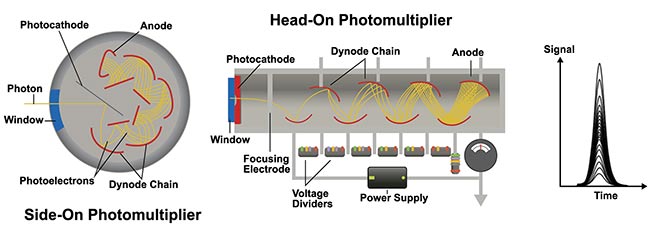
Figure 1. The input-output characteristics of the structure of a photomultiplier tube (PMT). When photons are incident on the photocathode, emitted electrons from the photocathode are amplified in a vacuum tube. As secondary electrons are repeatedly amplified at multiple dynode chains, the output pulse signal when detecting one photon is not uniform or stable. Courtesy of Evident Scientific.
Figure 2 shows the challenges of collecting varying fluorescent signal using a PMT. When the PMT gain is set high (top), a low intensity fluorescent signal (a small number of photons) can be detected. However, the output will be easily saturated, resulting in a small dynamic range. However, if the gain is low, the output signal will not be saturated even when strong fluorescence (many photons) is detected, equating to a higher dynamic range. But weak fluorescence is buried in the noise and will not be amplified, causing the signal-to-noise ratio (SNR) to deteriorate (bottom), obscuring relevant features and data in a sample. This variability in dynamic range and SNR therefore makes quantification exceedingly difficult because we cannot see all our fluorescent signal at once.
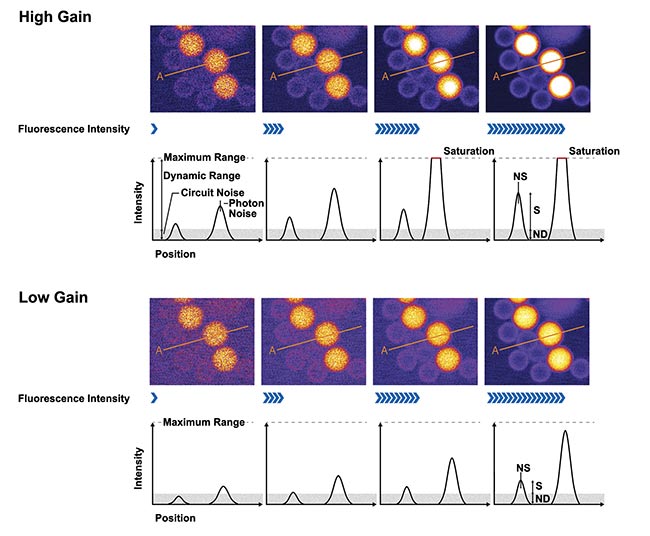
Figure 2. Adjusting the gain of a photomultiplier tube (PMT) requires balancing the signal-to-noise ratio (SNR) and dynamic range, which can be difficult. The images were acquired using different excitation laser settings; the images on the right were acquired using a higher setting. The plots below the images show the intensity profile along line A. The SNR is the ratio of S (the profile height) and NS (photon noise) and ND (circuit noise). The top shows samples acquired using high gain. The dim beads have a higher SNR, but the brighter beads get saturated. The bottom shows samples acquired using low gain. The dim beads have a lower SNR, but the bright beads do not get saturated. Courtesy of Evident Scientific.
Another issue that affects the use of PMTs in effective photon counting is that their sensitivity deteriorates over time, according to the accumulated detected photons by usage. When photons enter the photocathode, electrons are emitted from the photocathode into the vacuum tube due to the external photoelectric effect. The photocathode deteriorates because the electrons cannot be fully replenished. The dynodes will also degrade due to collision with the electrons emitted from the photocathode. This gradual degradation leads to a difference in intensity quantification over time, further limiting a PMT’s ability to quantify photons.
Silicon photomultiplier advantages
The integration of a silicon photomultiplier (SiPM) into a microscopic system eliminates many of the issues and restrictions of conventional PMTs (Figure 3). Geiger mode allows one-photon incidence to be detected at high signal levels by a highly stable multiplication process despite high gain. Furthermore, the semiconductor manufacturing process allows for precise control over the individual variations of SiPMs that affect sensitivity. Through consistent mass production, the differences in photodetection efficiency and gain between SiPMs can be minimized. In addition, even if many photons are incident at the same time, the sum of the respective avalanche photodiode currents is output from the SiPM, so the upper limit of the output current is high, resulting in a wide dynamic range to detect many incident photons. In other words, one photon signal can be multiplied with high gain and has a wide detection range.
These advantages make the SiPM an ideal candidate for a truly quantitative fluorescent detector that can measure activity within a cell.
This capability enables the SiPM to achieve a high SNR and a wide dynamic range simultaneously, eliminating the need to compromise between the two by adjusting the gain. In addition, photoelectric conversion by an SiPM, like photodiodes, uses the internal photoelectric effect, during which electrons are excited from the valence band to the conductor. Therefore, electrons are replenished quickly when they are excited. The result is that the sensitivity and gain are not degraded, even if there is a large amount of incident light. These advantages make the SiPM an ideal candidate for a truly quantitative fluorescent detector that can measure activity within a cell.
High-speed sampling
As described above, conventional systems balance the SNR and temporal resolution by combining signal smoothing using analog circuit filtering with the minimum necessary analog-to-digital (AD) sampling frequency (a sampling period of about one-half of the pixel period) for pixel resolution. However, this solution was technically limited to responding to the higher pixel number (shorter pixel period) by the high-speed resonant scanner, obscuring relative information from a sample.
New advancements in hardware enable it to realize a 1-GHz AD sampling rate, which is 12× faster than the conventional sampling rate, and to adopt an oversampling method in which a large amount of sampling is performed within one pixel period. All confocal imaging applications will be faster as a result, including imaging cellular dynamics. Since an SiPM sensor output has a wide dynamic range, the range of its output signal is also very large compared to a PMT. Along with the higher AD sampling rate, the amplitude-resolving accuracy is 16× higher (from 10 bit to 14 bit) than conventional devices. These high-performance devices are optimized for SiPM signal processing applications.
Noise isolation uses a digital-signal-processing filter instead of an analog-circuit filter, which efficiently attenuates noise while minimizing the sacrifice of the signal bandwidth to achieve a higher SNR. As a result, high-frequency components within an image that could not be separated by the conventional method can be detected separately, and sufficient pixel resolution (temporal resolution) can be achieved, even if the pixel number of the resonant scanner is 1K or larger.
Eliminating signal decay
While an SiPM sensor can output the photon detection timing and the number of photons detected accurately and quickly, it has one disadvantage — a slowly decaying output signal that lasts >200 ns (Figure 3b). When imaging using a high-speed resonant scanner, the short pixel dwell time causes the leakage of a decay signal into adjacent pixels, which degrades the pixel resolution and temporal resolution. This represents a significant problem for high-speed imaging of cellular dynamics, for example.
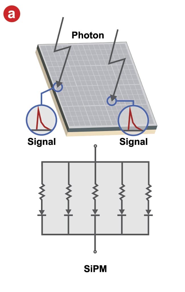
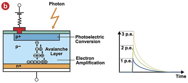
Figure 3. The structure of a silicon photomultiplier (SiPM) sensor and its input-output
characteristics. An SiPM is comprised of multipixel avalanche photodiodes (a). When
multiple photons are incident simultaneously, the output signal is the sum of the
avalanche photodiode signal (b). Courtesy of Evident Scientific.
Using advanced signal processing with a field programmable gate array (FPGA) allows the bandwidth degradation to be restored due to this slow signal decay. Raw SiPM output signals are more prone to pile up when high-frequency photon-detection events occur, such as the detection of more photons prior to the decay of the signal (blue line in Figure 4). Therefore, to take advantage of an SiPM's high dynamic range, the AD converter’s conversion scale must be larger than the signal amplitude of high-frequency photon detection, including the pile-up effect.
On the other hand, to perform the inverse transformation process accurately, the signal amplitude of one photon, which is the smallest signal, must be detected with a fine resolution pitch. Thus, an AD converter with higher resolution is required to capture smaller amplitudes with finer resolution and larger pile-up amplitudes. In addition, inverse transformation is impossible without very high time resolution, i.e., many digital data sequences acquired at fast sampling rates. Generally, AD converters with a 1-GHz sample rate for high-speed devices have an 8-bit degree of resolution. As shown in Figure 4, it is possible to achieve this inverse transformation process by using high-end AD converters with a 1-GHz sample rate, 14-bit resolution (16,384 gradation), and high-speed processing of the large-capacity, high-speed digital data obtained from these converters using a high-end FPGA.
As shown in Figure 4, if no inverse transformation occurs, the image pixel resolution will be degraded by the effect of the SiPM signal decay, particularly during high-speed and high-resolution resonant scanning, such as the real-time imaging of live organisms. On the other hand, applying the inverse transformation restores the temporal resolution without losing the photon input, enabling it to obtain a high-resolution resonant scanner image (1024 pixels/line) without the loss of spatial resolution or detected photons. This will allow researchers to capture fast dynamic events, such as calcium spikes at dendritic spines, with more clarity and precision.
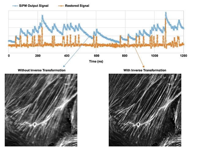
Figure 4. A sample captured with and without inverse transformation (Actin (BODIPY FL)) in a BPAE cell; resonant, average 64, ex. 488 nm, Em. 500 to 540 nm, same excitation power; UPLSAPO40x2/NA 0.95, CA 1 AU, 1024 × 1024 pixels. Courtesy of Evident Scientific.
HDR photon counting
The advanced signal processing discussed above indicates that the inversely transformed signal is restored, maintaining the time resolution by removing the decay signal (orange line in Figure 4). By leveling the piled-up signals, the pulse-output amplitude (wave peak value) corresponding to the detected number of photons can be obtained. In other words, when one photon is detected, pulses with the same amplitude are output. Similarly, when two photons are simultaneously detected, pulses with an amplitude twice as high are output.
If photons are simultaneously detected thereafter, the pulses are output with an amplitude that is an integer multiple of that one photon. Therefore, if N photons are detected within a certain time interval, the time integration of these output pulses can be obtained as the integrated intensity of N × the pulse at the time of one photon detection. This relationship also holds true when a large number of photons are detected within a very short time.
Consequently, this method enables the accurate detection of fluorescent light, even when a large number of photons are detected in a short period of time. Practically up to 1 gigaphoton per second can be detected with this SNR without saturation, enabling linearity at a high photon number. While the conventional single-photon counting detection method (paralytic or non-paralytic) could only be applied at low-frequency photon detection rates, the present technique achieves high dynamic range photon counting, which is comparable in SNR to the photon counting detection method, even when imaging very bright samples at high speeds (Figure 5).
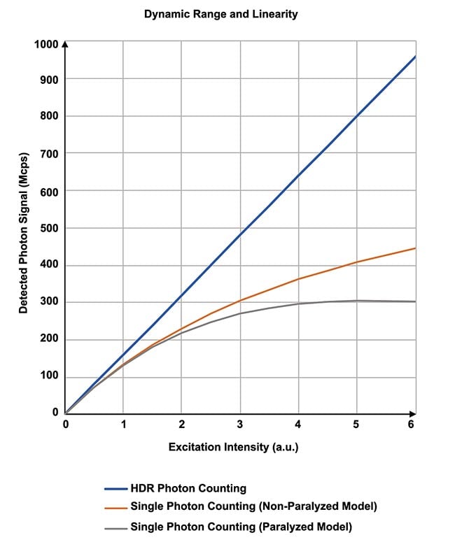
Figure 5. The relationship between excitation intensity and the output signal. Courtesy of Evident Scientific.
Dynamic range is limited in conventional PMT imaging; if the sample has a mix of dark and bright objects, one of them must be prioritized. For example, in Figure 6, when acquiring an image of neurons, intensity saturation at the cell body was inevitable to acquire clear images of the neural fiber's structure with weak fluorescence. By realizing high dynamic range photon counting, an SiPM with advanced signal processing can acquire both bright and dark areas without saturation.
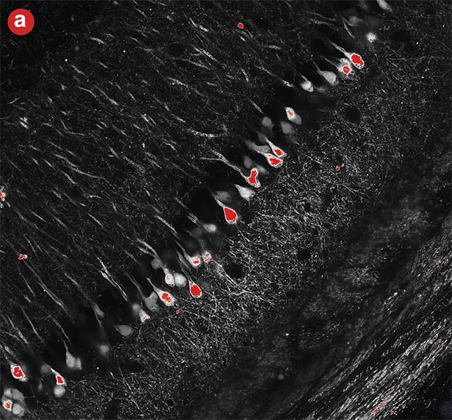
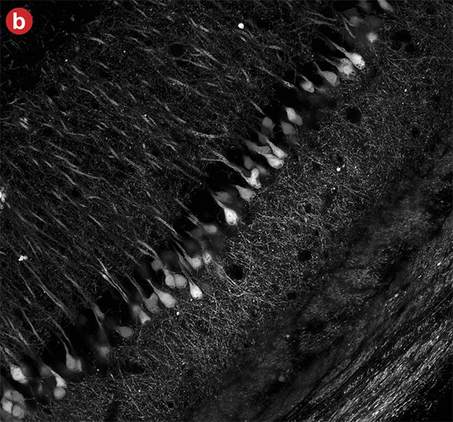
Figure 6. High dynamic range (HDR) imaging. A conventional photomultiplier tube (PMT) image in which the brighter neural cell bodies easily get saturated (a). An image captured using a silicon photomultiplier (SiPM) detector with advanced signal processing where both the cell body and neural fibers were in the detection range (b). Courtesy of Evident Scientific.
Figure 7 is a comparison of images and intensity measurements from a conventional PMT and an SiPM with advanced signal processing. Four points with varying photon numbers are measured in the same spot on both images. The PMT can only measure intensity, while the SiPM can register an exact photon count. Due to the physical properties of the SiPM, as well as the high sampling frequency, there is less background with the SiPM, as well. The increased dynamic range and lower noise lead to a higher SNR with the new detector technology.
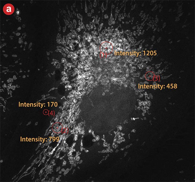
Figure 7. High dynamic range (HDR) photon counting. An image taken with a conventional photomultiplier tube (PMT) (a). The same area imaged using a silicon photomultiplier (SiPM) detector with HDR photon counting (b). The same areas are highlighted and measured on each image. Courtesy of Evident Scientific.
An ideal detector can relate the amount of detected fluorescence and the intensity on a quantitative scale. However, using conventional technology, this relationship is unclear and uncertain. Combining advanced signal processing hardware with an SiPM detector, it is now possible to quantify the amount of detected fluorescence using a clear quantitative scale — the number of photons.
With newer developments in imaging hardware available in many lasers’ scanning confocal systems, researchers can capture fast dynamic events, such as calcium spikes at dendritic spines with more clarity and precision. Essentially, this new technology will pave the way to transforming the capabilities of microscopy imaging.
Meet the authors
George Glekas, Ph.D., is a national applications specialist at Evident Scientific, focusing on laser scanning systems. He received his Ph.D. in biochemistry from the University of Illinois, studying chemotaxis. Further postdoctoral work at the University of North Carolina was heavily focused on developing novel biosensors. He has been with Evident Scientific since 2016 and is responsible for training, applications support, and new product development; email: george.[email protected].
Joanna Hawryluk, Ph.D., is a product manager for research imaging at Evident Scientific. She received her doctorate from the University of Connecticut within the Department of Physiology and Neurobiology. She has been with Evident since 2017, supporting research microscopy, and is currently responsible for the FLUOVIEW FV4000/FV4000MPE laser scanning microscopes; email: [email protected].