Prioritizing the key parameters for selecting the best grating for spectroscopic applications.
David Ventola, Optometrics Corp., an Omega Optical Holdings company
Diffraction gratings are optical components with a periodic structure that separate light into beams traveling in predictable directions based on their wavelength. The grating acts as the dispersive element at the heart of many modern spectroscopic instruments. They provide the critical function of selecting the wavelengths of light required to perform the analysis at hand. Selecting the best grating for an application is not difficult, but it will usually require some level of decision-making when prioritizing the key parameters for the application.
Any spectroscopic application will have at least two basic system requirements: It must be able to analyze material over the required spectral range of interest, and it must be able to provide sufficiently small spectral bandwidth to resolve the features of interest. These two key requirements form the foundation of the grating selection. The other grating properties are then chosen to optimize the performance within these basic constraints.
Grating basics
A surface-relief diffraction grating is a passive optical component that redirects light incident upon the surface at an angle that is unique for each wavelength in a given order. This redirection, or diffraction, is a result of the phase change of the electromagnetic wave as it encounters the regular, fixed structure of the grating surface. Each wavelength undergoes a different phase shift, and, as a result, reconstructs at a different angle, resulting in the dispersion of broadband light. If the wavelength of the incident radiation is much larger than the groove spacing, diffraction will not occur. If the wavelength is much smaller than the groove spacing, the facets of the groove will act as mirrors and, again, no diffraction will take place.
Grating types
The two most common groove profiles are referred to as ruled and holographic (Figures 1-6), which relates to the method in which the master grating was produced. Physically forming grooves into a reflective surface with a diamond tool using a ruling engine produces ruled gratings. Ruled grating groove profiles are very controllable and easy to optimize for a given application, and, in most cases, will provide the best diffraction efficiency due to this freedom.
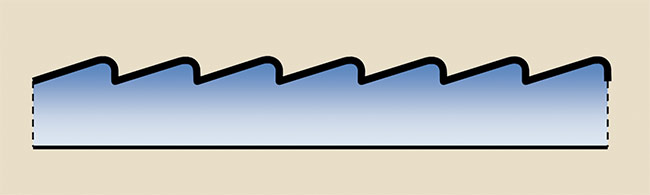
Figure 1. A typical profile of a ruled blazed grating.
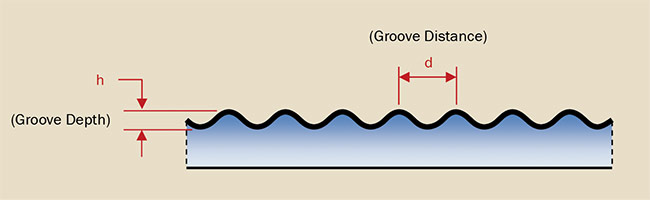
Figure 2. A symmetric profile of a holographic diffraction grating.
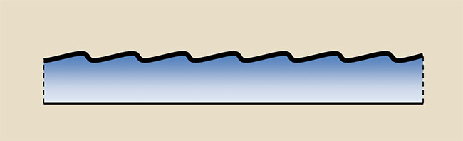
Figure 3. An asymmetric profile of a (blazed) holographic diffraction grating.
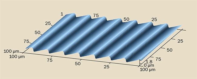
Figure 4. An actual measured profile of a coarse ruled blazed grating.
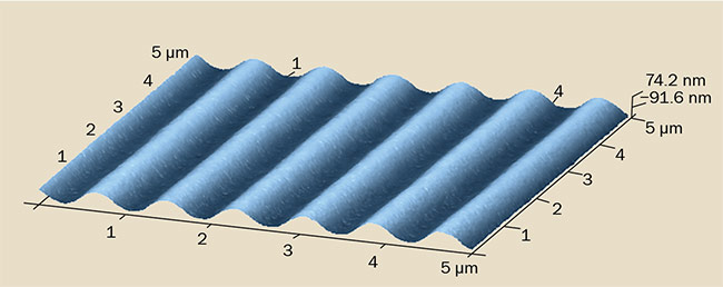
Figure 5. An actual measured profile of a symmetric holographic diffraction grating.
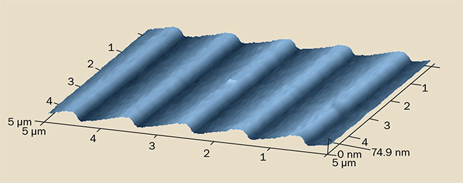
Figure 6. An actual measured profile of a blazed holographic diffraction grating.
Holographically produced groove profiles are generated interferometrically in photoresist and then transferred to durable materials for reproduction. Advantages of holographically generated gratings are that they minimize stray light and allow the production of groove spacings that, although possible, would be impractical using the ruling process in which the grooves are formed individually. For these reasons, holographic gratings predominate applications requiring UV wavelength analysis. With some notable exceptions, however, holographic gratings will generally have less peak diffraction efficiency than their ruled counterparts because their features are less abrupt and there are fewer degrees of freedom in control of the groove profile.
Dispersion, resolution, and resolving power
The primary function of a diffraction grating in a spectroscopic instrument is to angularly separate a broadband source into a spectrum in which each wavelength has a known direction. This property is known as dispersion, and the equation that dictates the relationship between wavelength and angle is commonly referred to as the Grating Equation:
n λ = d (sin θ + sin θ’)
where n = the order of diffraction,
λ = the wavelength of light,
d = the distance between adjacent grooves,
θ = the angle of incidence with respect to the grating normal, and θ’ = the angle of diffraction with respect to the grating normal (Figure 7).
The equation for angular dispersion is:
dθ/dλ = n/dcosθ’
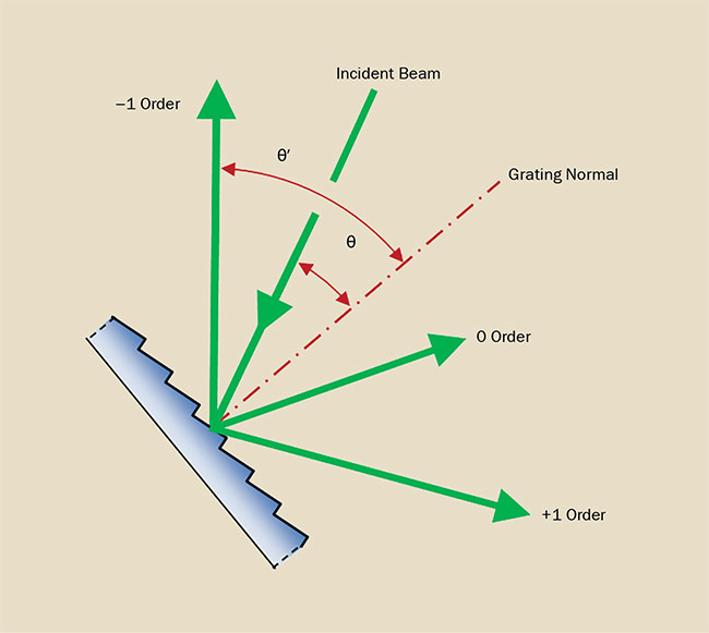
Figure 7. A typical diffraction pattern.
Resolution is a system property, not a grating property. A spectroscopic instrument must provide a spectral bandwidth narrow enough to distinguish the features of interest. This is accomplished through a combination of grating angular dispersion and system focal length, and by limiting aperture width. The spectral bandwidth at the detector plane can be equally accomplished with a low dispersion grating and a long focal length as with a high dispersion grating and shorter focal length. The limiting aperture in a system with a single element detector — for example, a scanning monochromator — is typically a physical slit with a known width. In a fixed grating spectrometer, the limiting aperture is typically an array element or camera pixel.
The equation for linear dispersion is:
dx/dλ = nF/dcosθ’
where F is the focal length of the
system.
Once the appropriate combination of focal length and grating dispersion is decided upon to accomplish the desired system resolution, one final test must be administered to ensure that the grating can provide the desired result. That is, to check that the grating has enough resolving power. Unlike resolution, resolving power is a property of the grating. The resolving power of a grating is given as:
λ/dλ = Nn
where N = the minimum number of grooves that the light must hit.
In simple terms, to resolve 1 nm at 1 µm (1000:1), there must be at least 1000 grooves. This limitation usually is not present, so it is easy to overlook, but it does provide a limit on how small the beam can be, or how coarse the groove spacing can be, for a given application. Keep in mind that all of these equations define the theoretical limits of what can be accomplished under ideal conditions, and that real life conditions such as image distortion will degrade the actual performance.
Efficiency
Once the appropriate groove spacing has been determined, the grating selection process becomes much easier. Assuming that the grating spacing is capable of covering the entire spectral range of interest, diffraction efficiency curves (Figure 8) are readily available for most popular gratings as a starting point. Select the grating that provides the best efficiency at the wavelengths that need it the most. This will require factoring in other elements of the system, such as the sample, source intensity profile, and detector responsivity.
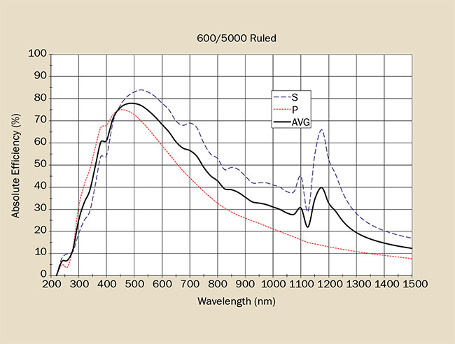
Figure 8. A typical grating efficiency curve.
The absolute efficiency of a grating is the percentage of incident monochromatic radiation that is diffracted into the desired order. In contrast, relative efficiency compares the energy diffracted into the desired order with that of a plane mirror coated with the same material as the grating. When comparing grating performance curves, it is important to keep this in mind. A relative efficiency curve will always show higher values than an absolute efficiency curve for the same grating.
Grating efficiency curves typically are measured with the grating in Littrow, or near-Littrow conditions. In the Littrow mounting configuration, the diffracted order and wavelength of interest are directed back along the path of the incident light. This geometry is rarely utilized in actual practice but is a standard by which grating performance can be compared equally. Most applications will require some deviation angle between the incident and diffracted beams. Small deviations from the Littrow mounting seldom have an appreciable effect on grating performance other than to slightly reduce the peak efficiency and limit the maximum wavelength achievable.
Blaze angle and wavelength
Grating efficiency is the product of groove shape and the reflectance of the coating, in the case of reflection gratings. The optimal groove shape is then determined by the angle of incidence.
The grooves of a ruled grating have a sawtooth profile with one side longer than the other. The angle made by a groove’s longer side and the plane of the grating is the “blaze angle.” Changing the blaze angle concentrates diffracted radiation to a specific region of the spectrum, increasing the efficiency of the grating in that region. The wavelength at which maximum efficiency occurs is the “blaze wavelength.” Classically, for ruled gratings, the blaze angle is calculated using the Grating Equation for the desired blaze wavelength in the Littrow mounting, where θ = θ’, so, by definition, it is only good for one wavelength at one angle in a mounting configuration that is rarely used in practice. Grating performance is always best judged by the measured efficiency curves. Small deviations from the ideal blaze angle and wavelength rarely have an appreciable effect on total performance.
Holographic gratings are not “blazed” in the classical sense. Their sinusoidal shape can, in some instances, be altered to approach the efficiency of a ruled grating. There are also special cases that should be noted. When the spacing-to-wavelength ratio is near one, a sinusoidal grating has virtually the same peak efficiency as a ruled grating. A holographic grating with 1800 g/mm can have the same efficiency at 500 nm as a blazed, ruled grating. In addition, special processes enable holographic gratings to achieve a sawtooth profile peaked near 240 nm — which is ideal for UV applications requiring good efficiency with low stray light.
Diffracted orders
For a given set of angles (θ, θ’) and groove spacing, the grating equation is valid at more than one wavelength, giving rise to several orders of diffraction. For example, 400-nm second-order radiation is diffracted from the grating at the same angle as 800-nm first-order radiation. The second-order light may need to be filtered to preserve the spectral purity at 800 nm. The measured intensity of the second order is a function of the source intensity of the lower wavelength, the detector sensitivity at that wavelength, and the second-order diffraction efficiency of the grating. At higher orders, the free spectral range decreases while angular dispersion increases (Figure 9). Order overlap can be compensated for by the judicious use of sources, detectors, and filters and usually is not a major problem in gratings used in low orders.
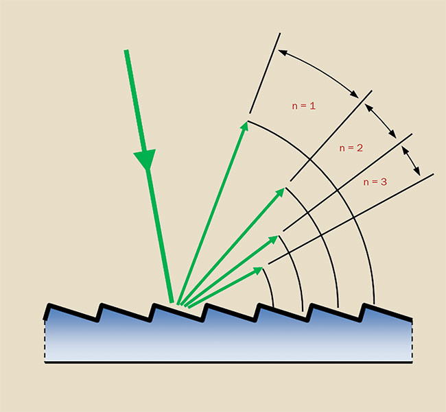
Figure 9. The free spectral range decreases with increasing diffraction order.
Free spectral range
Free spectral range is the maximum spectral bandwidth that can be obtained in a specified order without spectral interference (overlap) from adjacent orders. As grating spacing decreases, the free spectral range increases. It decreases with higher orders. If λ1 and λ2 are the lower and upper limits respectively of the band of interest, then:
the free spectral range = λ2 - λ1 = λ/n.
Coatings
Several reflective coatings (Figure 10) are used on reflection gratings, most commonly bare aluminum (Al), protected aluminum, and gold (Au). Bare aluminum is the most economical, and offers good reflectance in the UV, VIS, and IR. Protected aluminum consists of an aluminum coat with a thin overcoat of magnesium fluoride to prevent the formation of aluminum oxide on the surface of the aluminum, which is absorbing in the deep UV. Gold offers superior performance over aluminum in the NIR region of the spectrum, particularly between 700 and 1000 nm, where aluminum has a reflectance dip. Below 600 nm, the reflectance of gold falls off rapidly and is a poor choice for gratings required to work below this wavelength. Above 1200 nm, the reflectance curves of gold and aluminum nearly reconverge, and the gold has minimal advantage for a single-pass application.
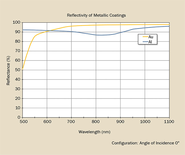
Figure 10. Aluminum (Al) versus gold (Au) reflectance.
Polarization
Gratings perform very differently in polarized light. If the incident light is randomly polarized, this is generally not a problem. The diffracted light will however exhibit some polarization bias after diffraction. This effect can range from very small to very large (Figures 11 and 12). The most effective way to minimize polarization effects is to keep the diffraction angles small. This usually means lowering the dispersion. Alternatively, utilizing a transmission grating rather than a reflection grating will nearly eliminate the effect. Transmission gratings generally have lower dispersion but also have the added advantage of the absence of metallic coatings, which are the main source of the effect. If the incident light is polarized, it is obviously very important to orient the polarization properly because there could be as much as a 10× difference in diffraction efficiency.
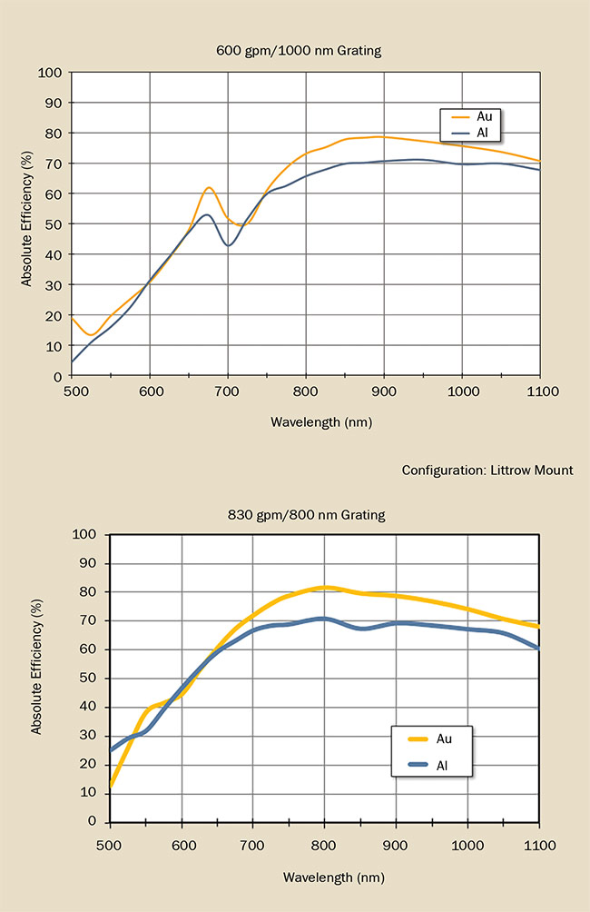
Figure 11. Two examples of the benefits of gold coating on NIR reflection gratings.
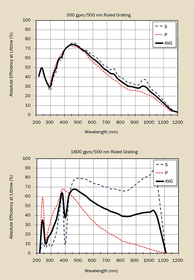
Figure 12. Examples of the relationship between dispersion and polarization sensitivity in reflection gratings.
Selection recommendations
A wide variety of diffraction gratings is commercially available to suit most applications. The vast majority of these gratings are produced as replicas of one master grating. While replica gratings are affordably priced, the master gratings that produce them are expensive to produce. Custom grating designs should be considered only when necessary.
The following are some additional helpful suggestions:
Do’s
1. Always use a commercially available grating whenever possible. This will always be the most economical solution.
2. Always consult a qualified grating manufacturer for a recommendation or for answers to any questions. The manufacturer can usually estimate the performance versus the cost benefit of a custom design if what is currently available is not a perfect match for an application. In many cases, the gains from an optimized design are minimal.
3. Call the manufacturer if published information is not optimum for your needs. Typically, what is published is only a sampling of what is available.
4. Allow for some production variation. Published performance information is representative only. Individual part testing is achievable but costly.
Don’ts
1. Do not over-tolerance the mechanical dimensions, particularly the thickness. Although tight tolerances are achievable, glass processing methods are completely different from metal machining techniques.
2. Do not assume theoretical performance. While grating performance modeling programs are very useful for comparative analysis and design optimization, they usually assume perfect materials and groove shape. A high-quality replica grating will generally yield between 80% and 95% of theoretical performance for most performance parameters.
3. Avoid the temptation of assuming that a ruled grating profile will not provide acceptable stray light performance. Modern interferometric controls have virtually eliminated the mechanical errors associated with ruling engines. The majority of the scattered light from a grating is due to surface roughness, which has as much to do with the quality of the replication process as the actual method of master production.
4. If a custom grating design is warranted, try to limit ruled-grating groove frequency to ~1500 mm or less. Higher groove frequencies are certainly achievable, but the grooves are formed one at a time, and higher frequencies can sometimes take weeks to produce a large master.